Basic Plotting With ggplot2

Introduction to R For Biologists and Bioinformatics

Dr Stevie Pederson

Black Ochre Data Labs
Telethon Kids Institute

September 19, 2023

Basic Data Visualisation

Data Visualisation

  • Now we know how to import data
    \(\implies\) what does it look like?
  • Traditionally R used functions from base and graphics
  • The main plotting package from the tidyverse is ggplot2
    • Incredibly powerful approach to plotting
    • Uses an approach known as “Grammar of Graphics” (gg)
  • Less intuitive than traditional R plots
    • Far simpler after some practice
    • Much more powerful

Setup For This Section

  1. Clear your R Environment
  2. Create a new R script called basic_ggplot.R
  3. Copy the following chunk from the earlier section
library(tidyverse)
pigs <- read_csv("data/pigs.csv")
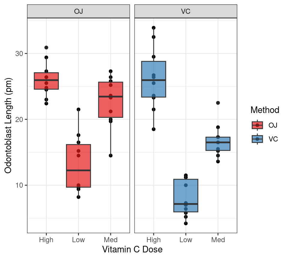
glimpse(pigs)
Rows: 60
Columns: 3
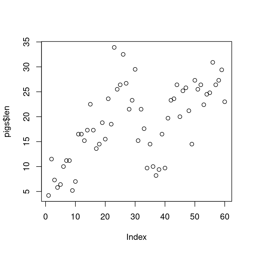
$ len  <dbl> 4.2, 11.5, 7.3, 5.8, 6.4, 10.0, 11.2, 11.2, 5.2, 7.0, 16.5, 16.5,…
$ supp <chr> "VC", "VC", "VC", "VC", "VC", "VC", "VC", "VC", "VC", "VC", "VC",…
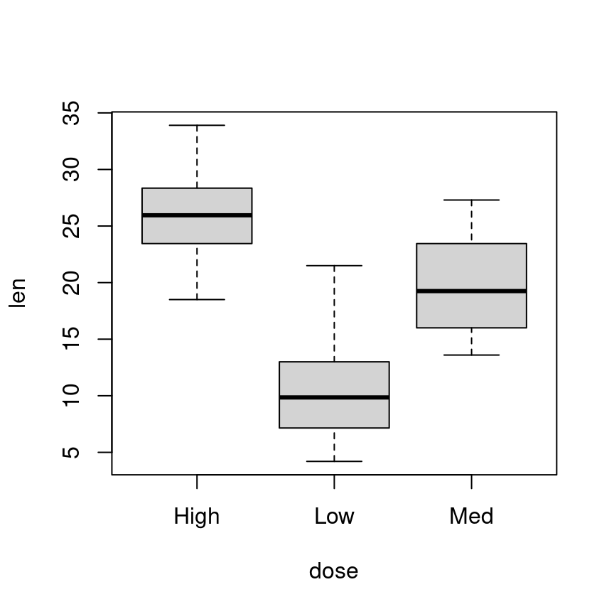
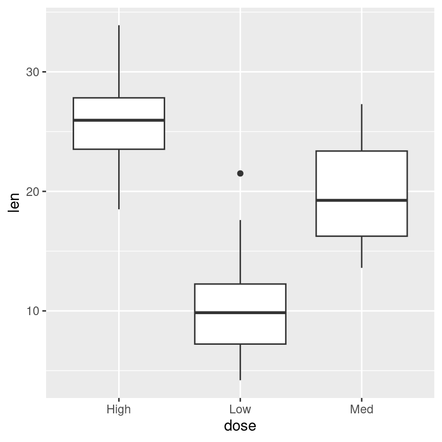
$ dose <chr> "Low", "Low", "Low", "Low", "Low", "Low", "Low", "Low", "Low", "L…

Plotting using base

plot(pigs$len)

This has plotted tooth length (len) in the order of appearance

Plotting using base

  • We can make boxplots using the formula syntax len ~ dose
    \(\implies\) len “depends on” dose
    • The predictor variable (dose) on the x-axis
    • The response variable (len) on the y-axis
boxplot(len ~ dose, data = pigs)

Histograms

  • Histograms using hist() can be pretty useful
hist(pigs$len)

Using ggplot2

ggplot2 Basics

Instead of a single function \(\implies\) build a plot using layers

  1. Start by defining the data object
    • Values for x & y axes usually defined here
  2. Add layers defining the geometry to use
    • May be points (geom_point), boxplots (geom_boxplot) etc
  1. Optionally split into panels or facets
  2. Optionally modify any scales used
  3. Optionally tidy up labels
  4. Optionally define an overall plotting theme

A simple boxplot

  • What values are the response variable? len
  • What values are the predictor variable? Either dose or supp
  • Let’s start putting dose on the x-axis

A simple boxplot

ggplot(pigs, aes(x = dose, y = len))

  • We haven’t added any geometry so none is drawn
  • We defined the values to be placed on x and y \(\implies\) axes were drawn
    • These were defined as aesthetic mappings using aes()

A simple boxplot

  • Geometry is added by
    1. Placing a + at the end of the first line
    2. Calling a geom_* function, e.g. geom_boxplot()
ggplot(pigs, aes(x = dose, y = len)) +
  geom_boxplot()

Using Colours

  • We can add more mappings to aes()
    • Show the supplement method as the boxplot fill
ggplot(
  pigs, aes(x = dose, y = len, fill = supp)
) +
  geom_boxplot()

Using Colours

  • We can change the palette using scale_fill_*
ggplot(
  pigs, aes(x = dose, y = len, fill = supp)
) +
  geom_boxplot() +
  scale_fill_brewer(palette = "Set1")

scale_fill_*()

  • There are multiple options for defining colour palettes (i.e. scales)
    • scale_fill_discrete() is applied by default
    • scale_fill_viridis_d() (_d for discrete)
    • scale_fill_grey()
    • scale_fill_manual()
  • We will explore more of these as we learn more
  • The difference between discrete & continuous values is important
  • Colour/Fill palettes:
    • colour is for shape outlines
    • fill is for filled shapes

Using Existing Themes

  • We can get rid of the horrible grey background using a theme()
ggplot(
  pigs, aes(x = dose, y = len, fill = supp)
) +
  geom_boxplot() +
  scale_fill_brewer(palette = "Set1") +
  theme_bw()

theme_bw()

  • theme_bw() is my default for how plots look
    • theme_grey() is the default
    • Other complete themes: theme_classic(), theme_minimal()
  • Adding theme() can modify the overall layout
    • legend.position, legend.justiication
    • axis.text, axis.tixks
    • panel.background
  • Very powerful and we’ll explore more later

Labels

  • Tidy up labels for aesthetic mappings
ggplot(
  pigs, aes(x = dose, y = len, fill = supp)
) +
  geom_boxplot() +
  scale_fill_brewer(palette = "Set1") +
  labs(
    x = "Vitamin C Dose", 
    y = "Odontoblast Length (pm)", 
    fill = "Method"
  ) +
  theme_bw() 

Facets

  • We could even show each method in it’s own panel (i.e. facet)
ggplot(
  pigs, aes(x = dose, y = len, fill = supp)
) +
  geom_boxplot() +
  facet_wrap(~supp) +
  scale_fill_brewer(palette = "Set1") +
  labs(
    x = "Vitamin C Dose", 
    y = "Odontoblast Length (pm)", 
    fill = "Method"
  ) +
  theme_bw() 

Different Geometries

geom_*()

  • Multiple options for geometry exist
    • Points: geom_point(), geom_jitter()
    • Bar-plots: geom_col(), geom_bar()
    • Boxplots: geom_boxplot(), geom_violin()
    • Distributions: geom_density(), geom_histogram()
    • Lines: geom_line(), geom_path()
    • Straight Lines: geom_abline(),geom_hline(), geom_vline()
    • Short Line Segments: geom_errorbar(), geom_segment()
    • Text: geom_text(), geom_label()
    • Heatmaps: geom_rect(), geom_raster(), geom_tile()

Overlaying points

  • Add geom_point() with some transparency (alpha) to the boxplot fill
    • Will be drawn before the boxplot (i.e. in order of the code)
ggplot(
  pigs, aes(x = dose, y = len, fill = supp)
) +
  geom_point() +
  geom_boxplot(alpha = 0.7) +
  facet_wrap(~supp) +
  scale_fill_brewer(palette = "Set1") +
  labs(
    x = "Vitamin C Dose", 
    y = "Odontoblast Length (pm)", 
    fill = "Method"
  ) +
  theme_bw() 

Overlaying points

  • geom_jitter() is geom_point() with a bit of noise added
    • width & height control x & y noise respectively
ggplot(
  pigs, aes(x = dose, y = len, fill = supp)
) +
  geom_jitter(width = 0.1, height = 0) +
  geom_boxplot(alpha = 0.7) +
  facet_wrap(~supp) +
  scale_fill_brewer(palette = "Set1") +
  labs(
    x = "Vitamin C Dose", 
    y = "Odontoblast Length (pm)", 
    fill = "Method"
  ) +
  theme_bw() 

Additional Comments

Categorical Variables

  • dose and supp are categorical variables (i.e. discrete)
    • Known in R as factors
    • By default, levels are assigned in alphabetic order
    • We’ll learn more about these in the next section

NB

  • ggplot is the function
  • ggplot2 is the package name
  • Hadley started with ggplot as the package name
    • Abandoned and rewrote as ggplot2 during his PhD
    • Probably would’ve done things differently in hindsight
  • The package ggplot is not publicly available

Conclusion

  • Beyond the first boxplot
    \(\implies\) can be very difficult to draw using base/graphics
  • The dataset determines what geometry is appropriate
  • Highly customisable plots
    • Colour/Fill palettes
    • Scales for axes can be log transformed, trimmed etc
    • Themes control overall appearance
  • All take a while to learn
    • Practice, practice, practice
    • The R Graphics Cookbook is a free online resource