Basic Statistics in R

RAdelaide 2024

Dr Stevie Pederson

Black Ochre Data Labs
Telethon Kids Institute

July 10, 2024

Statistics in R

Introduction

R has it’s origins as a statistical analysis language (i.e. S)
Purpose of this session is NOT to teach statistical theory
- I am a bioinformatician NOT a statistician
Perform simple analyses in R
Up to you to know what you’re doing
- Or talk to your usual statisticians & collaborators

Distributions

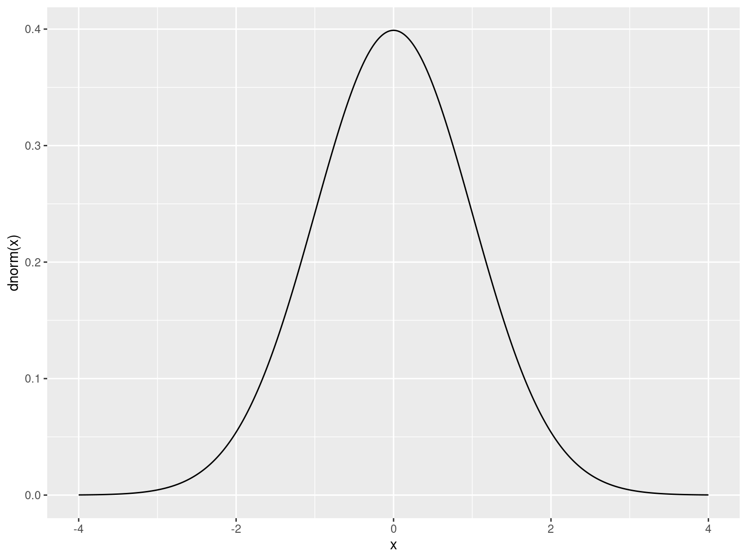
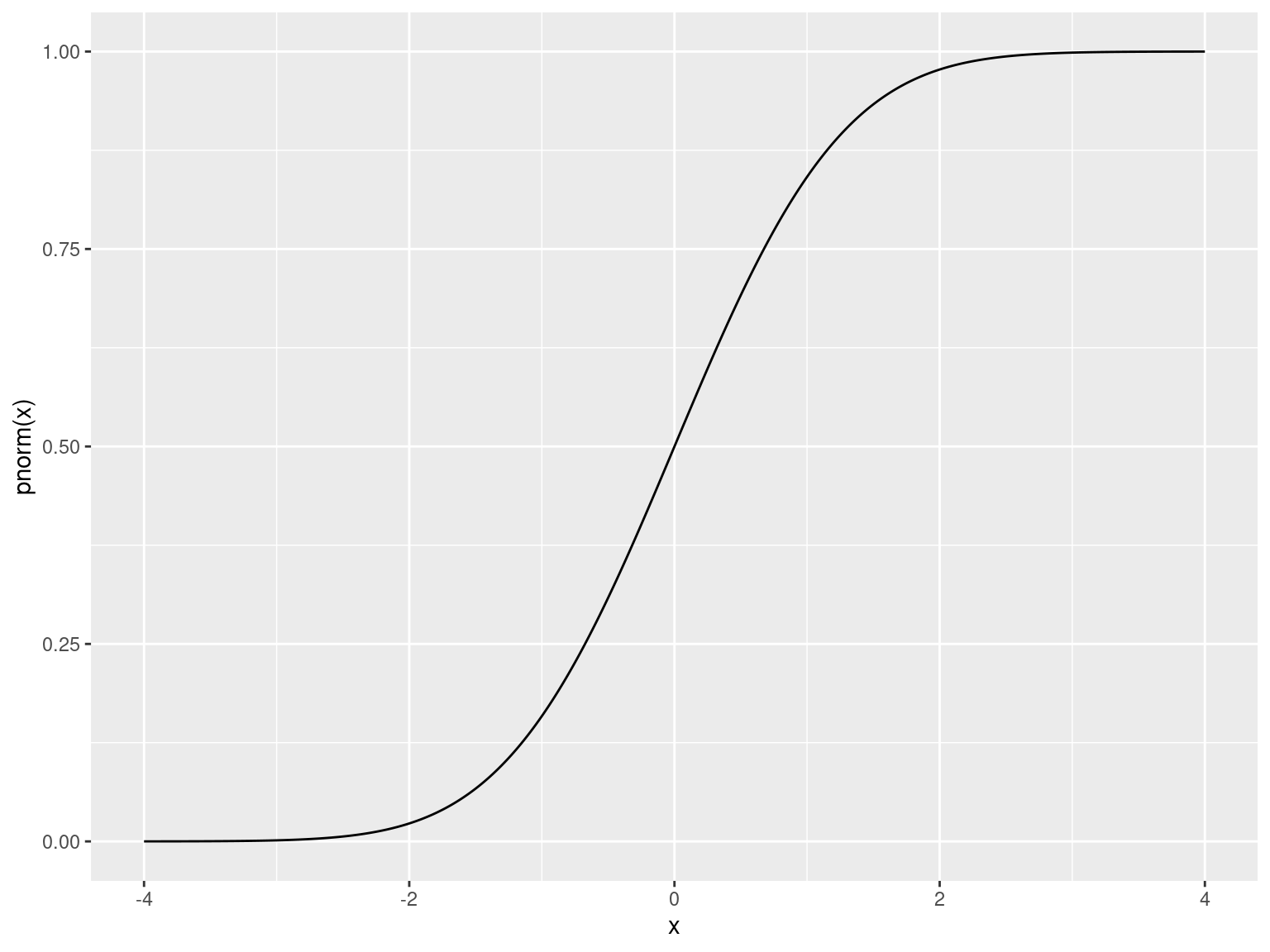
R comes with nearly every distribution
Standard syntax for accessing each

Distributions

Distribution	Density	Area Under Curve	Quantile	Random
Normal	`dnorm()`	`pnorm()`	`qnorm()`	`rnorm()`
T	`dt()`	`pt()`	`qt()`	`rt()`
Uniform	`dunif()`	`punif()`	`qunif()`	`runif()`
Exponential	`dexp()`	`pexp()`	`qexp()`	`rexp()`
$\chi^2$	`dchisq()`	`pchisq()`	`qchisq()`	`rchisq()`
Binomial	`dbinom()`	`pbinom()`	`qbinom()`	`rbinom()`
Poisson	`dpois()`	`ppois()`	`qpois()`	`rpois()`

Distributions

Also Beta, $\Gamma$, Log-Normal, F, Geometric, Cauchy, Hypergeometric etc…

?Distributions

Distributions

## dnorm gives the classic bell-curve
tibble(
  x = seq(-4, 4, length.out = 1e3)
) %>% 
  ggplot(aes(x, y = dnorm(x))) + 
  geom_line()

## pnorm gives the area under the 
## bell-curve (which sums to 1)
tibble(
  x = seq(-4, 4, length.out = 1e3)
) %>% 
  ggplot(aes(x, y = pnorm(x))) + 
  geom_line()

Basic Tests

Data For This Session

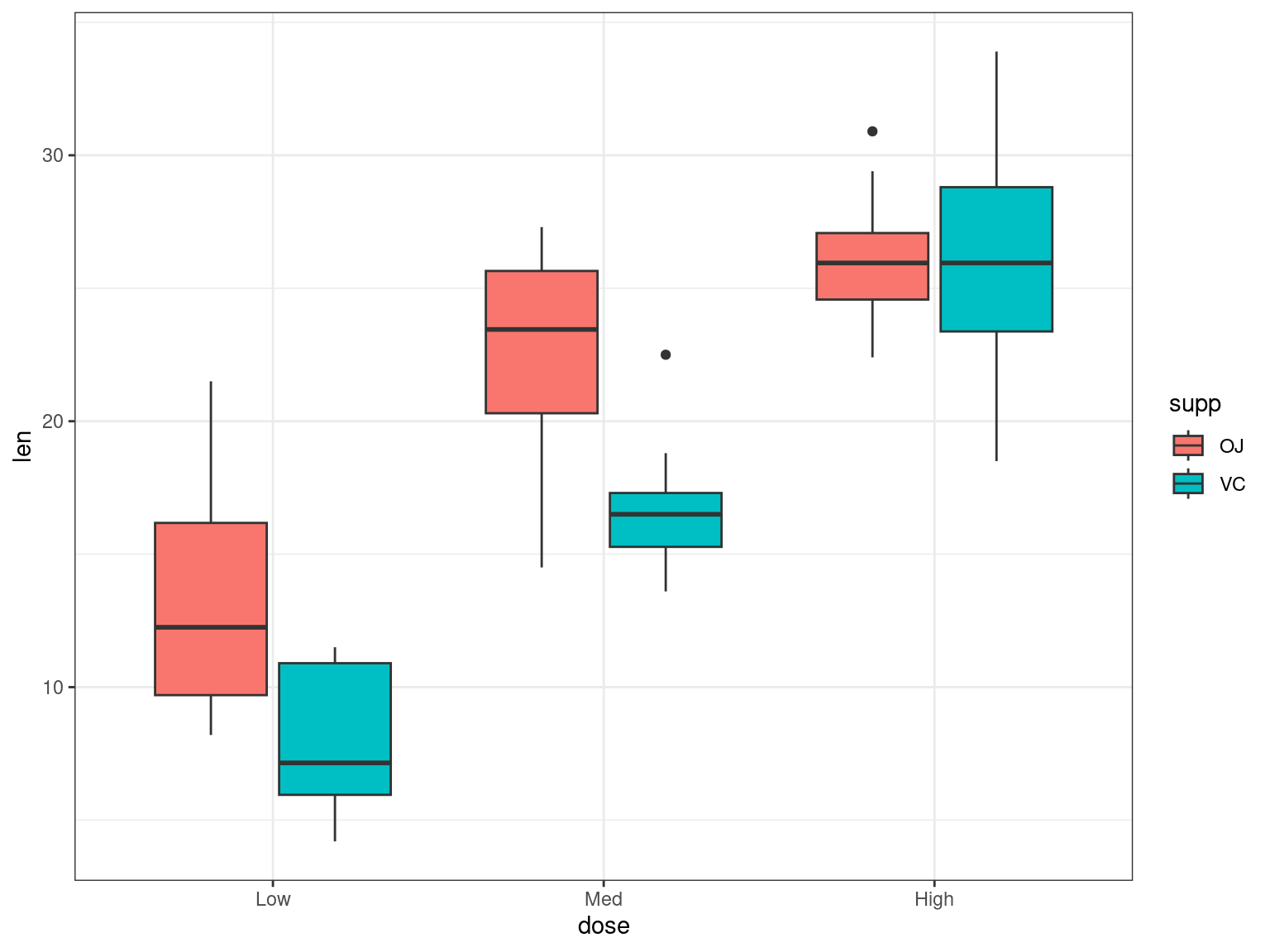
We’ll use the pigs dataset from earlier

library(tidyverse)
pigs <- file.path("data", "pigs.csv") %>%
    read_csv %>%
    mutate(dose = factor(dose, levels = c("Low", "Med", "High")))

Data For This Session

theme_set(theme_bw())
pigs %>% 
  ggplot(
    aes(x = dose, y = len, fill = supp)
  ) +
    geom_boxplot()

t-tests

Assumes normally distributed data
$t$-tests always test $H_0$ Vs $H_A$

The simplest test is on a simple vector
- This is not particularly meaningful for our data

?t.test
t.test(pigs$len)

What is $H_0$ in the above test?

t-tests

When comparing the means of two vectors

\[ H_0: \mu_{1} = \mu_{2} \\ H_A: \mu_{1} \neq \mu_{2} \]

We could use two vectors (i.e. x & y)

vc <- dplyr::filter(pigs, supp == "VC")$len
oj <- dplyr::filter(pigs, supp == "OJ")$len
t.test(x = vc, y = oj)

Is this a paired test?

t-tests

An alternative is the R formula method: len~supp
- Length is a response variable
- Supplement is the predictor
Can only use one predictor for a T-test
- Otherwise it’s linear regression

t.test(len~supp, data = pigs)

Did this give the same results?

Wilcoxon Tests

We assumed the above dataset was normally distributed:
What if it’s not?

Non-parametric equivalent is the Wilcoxon Rank-Sum (aka Mann-Whitney)

This assigns ranks to each value based on their value
- Tied values can be problematic
Values not used in calculation of the test statistic

wilcox.test(len~supp, data = pigs)

$\chi^2$ Test

Here we need counts
Commonly used in Observed Vs Expected

\[ H_0: \text{No association between groups and outcome}\\ H_A: \text{Association between groups and outcome} \]

$\chi^2$ Test

pass <- matrix(c(25, 8, 6, 15), nrow = 2)
colnames(pass) <- c("Pass", "Fail")
rownames(pass) <- c("Attended", "Skipped")
pass
chisq.test(pass)

Can anyone remember when we shouldn’t use a $\chi^2$ test?

Fisher’s Exact Test

$\chi^2$ tests became popular in the days of the printed tables
- We now have computers
Fisher’s Exact Test is preferable in the cases of low cell counts
- (Or any other time…)
Same $H_0$ as the $\chi^2$ test
Uses the hypergeometric distribution

fisher.test(pass)

Summary of Tests

t.test(), wilcox.test()
chisq.test(), fisher.test()

shapiro.test(), bartlett.test()
- Tests for normality or homogeneity of variance

binomial.test(), poisson.test()
kruskal.test(), ks.test()

`htest` Objects

All produce objects of class htest
Use print.htest() to display results
Is really a list
- Use names() to see what other values are returned

Can usually extract p-values using test$p.value

fisher.test(pass)$p.value

Regression

Linear Regression

We are trying to estimate a line with slope & intercept

\[ y = ax + b \]

\[ y = \beta_0 + \beta_1 x \]

Linear Regression

Linear Regression always uses the R formula syntax

y ~ x: y is a function of x
We use the function lm()

lm_pigs <- lm(len ~ supp , data = pigs) 
summary(lm_pigs)

Intercept is assumed unless explicitly removed (~ 0 + ...)

Linear Regression

It looks like supp == VC reduces the length of the teeth
In reality we’d like to see if dose has an effect as well

lm_pigs_dose <- lm(len ~ supp + dose, data = pigs) 
summary(lm_pigs_dose)

Which values are associated with the intercept & slope?

It looks like an increasing dose-level increases length

Interaction Terms

We have given each group a separate intercept
- The same slope
- Requires an interaction term for different slopes

lm_pigs_full <- lm(len ~ supp + dose + supp:dose, data = pigs) 
summary(lm_pigs_full)

How do we interpret this?

Interaction Terms

An alternative way to write the above in R is:

lm_pigs_full <- lm(len ~ (supp + dose)^2, data = pigs) 
summary(lm_pigs_full)

Model Selection

Which model should we choose?

anova(lm_pigs, lm_pigs_dose, lm_pigs_full)

Model Selection

Are we happy with our model assumptions?

Normally distributed
Constant Variance
Linear relationship

plot(lm_pigs_full)

Model Selection

This creates plots using base graphics
To show them all on the same panel

par(mfrow = c(2, 2))
plot(lm_pigs_full)

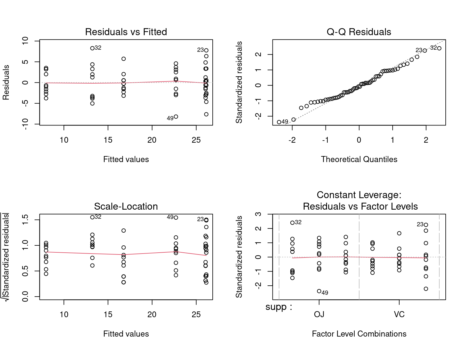
Visualising Residuals

mfrow() stands for multi-frame row
Needs to be reset to a single frame

par(mfrow = c(1, 1))

Logistic Regression

Logistic Regression models probabilities (e.g. $H_0: \pi = 0$)
We can specify two columns to the model
- One would represent total successes, the other failures
- This is binomial data, $\pi$ is the probability of success

Alternatively the response might be a vector of TRUE/FALSE or 0/1

Logistic Regression

The probability of admission to a PhD¹
- Graduate Record Exam scores
- Grade Point Average
- Prestige of admitting institution (1 is most prestigous)

admissions <- read_csv("https://stats.idre.ucla.edu/stat/data/binary.csv")
glimpse(admissions)

Rows: 400
Columns: 4
$ admit <dbl> 0, 1, 1, 1, 0, 1, 1, 0, 1, 0, 0, 0, 1, 0, 1, 0, 0, 0, 0, 1, 0, 1…
$ gre   <dbl> 380, 660, 800, 640, 520, 760, 560, 400, 540, 700, 800, 440, 760,…
$ gpa   <dbl> 3.61, 3.67, 4.00, 3.19, 2.93, 3.00, 2.98, 3.08, 3.39, 3.92, 4.00…
$ rank  <dbl> 3, 3, 1, 4, 4, 2, 1, 2, 3, 2, 4, 1, 1, 2, 1, 3, 4, 3, 2, 1, 3, 2…

Logistic Regression

glm(admit ~ gre + gpa + rank, data = admissions, family = "binomial") %>% 
  summary()


Call:
glm(formula = admit ~ gre + gpa + rank, family = "binomial", 
    data = admissions)

Coefficients:
             Estimate Std. Error z value Pr(>|z|)    
(Intercept) -3.449548   1.132846  -3.045  0.00233 ** 
gre          0.002294   0.001092   2.101  0.03564 *  
gpa          0.777014   0.327484   2.373  0.01766 *  
rank        -0.560031   0.127137  -4.405 1.06e-05 ***
---
Signif. codes:  0 '***' 0.001 '**' 0.01 '*' 0.05 '.' 0.1 ' ' 1

(Dispersion parameter for binomial family taken to be 1)

    Null deviance: 499.98  on 399  degrees of freedom
Residual deviance: 459.44  on 396  degrees of freedom
AIC: 467.44

Number of Fisher Scoring iterations: 4

Logistic Regression

Probabilities are fit on the logit scale
Transforms 0 < $\pi$ < 1 to $-\infty$ < logit($\pi$) < $\infty$

\[ \text{logit}(\pi) = \log(\frac{\pi}{1-\pi}) \]

Automated Model Selection

One strategy during model fitting is to fit a heavily parameterised model
R can remove terms as required using Akaike’s Information Criterion (AIC)
- The function is step()

glm(admit ~ (gre + gpa + rank)^2, data = admissions, family = "binomial") %>% 
  step() %>% 
  summary()

Here we do end up with the same model

Mixed Effects Models

Mixed effects models include:

Fixed effects & 2) Random effects

May need to nest results within a biological sample, include day effects etc.

Rabbit <- MASS::Rabbit
head(Rabbit)

Mixed Effects Models

Here we have the change in Blood pressure within the same 5 rabbits

6 dose levels of control + 6 dose levels of MDL
Just looking within one rabbit

filter(Rabbit, Animal == "R1")

Mixed Effects Models

If fitting within one rabbit $\implies$ use lm()

lm_r1 <- lm(
  BPchange~(Treatment + Dose)^2, data = Rabbit, subset = Animal == "R1"
)
summary(lm_r1)

Mixed Effects Models

To nest within each rabbit we:

Use lmer() from lme4
Introduce a random effect (1|Animal)
- Captures variance between rabbits

library(lme4)
lme_rabbit <- lmer(BPchange~Treatment + Dose + (1|Animal), data = Rabbit)
summary(lme_rabbit)
coef(summary(lme_rabbit))

Mixed Effects Models

This gives $t$-statistics, but no $p$-value

Why?

library(lmerTest)
lme_rabbit <- lmer(BPchange~Treatment + Dose + (1|Animal), data = Rabbit)
summary(lme_rabbit)

Mixed Effects Models

Doug Bates & Ben Bolker are key R experts in this field
- Doug has left the R community
Lots of discussion for issues estimating DF with random effects
Ben Bolker also maintains glmmTMB and glmmADMB
- Generalised Mixed-effects Models
- https://bbolker.github.io/mixedmodels-misc/glmmFAQ.html

Modelling Summary

lm() for standard regression models
glm() for generalised linear models
lmer() for linear mixed-effects models

Robust models are implemented in MASS

Other Statistical Tools

Mutiple Testing in R

The function p.adjust() takes the argument method = ...

p.adjust.methods

[1] "holm"       "hochberg"   "hommel"     "bonferroni" "BH"        
[6] "BY"         "fdr"        "none"

lm_pigs_full %>% 
  broom::tidy() %>% 
  mutate(
    adjP = p.adjust(p.value, "bonf"),
    sig = case_when(
      adjP < 0.001 ~ "***",
      adjP < 0.01 ~ "**",
      adjP < 0.05 ~ "*",
      adjP < 0.1 ~ ".",
      TRUE ~ ""
    )
  )

Also the package multcomp is excellent but challenging

PCA

Here we have 50 genes, from two T cell types: Both Stimulated & Resting ¹

genes <- read_csv("data/geneExpression.csv")

PCA requires a numeric matrix

gene_mat <- genes %>% 
  as.data.frame() %>% 
  column_to_rownames("ID") %>% 
  as.matrix()

PCA

Our variable of interest here is the cell-types
We need to set that as the row variable:
- Transpose the data using t()
- Default settings need tweaking (S reverse compatability)

pca <- gene_mat %>% 
  t() %>% 
  prcomp(center = TRUE, scale. = TRUE)
summary(pca)
biplot(pca)

screeplot(pca)

These plots aren’t great…

PCA

The output of prcomp() is a list with class prcomp
Components are in pca$x
Gene loadings are in pca$rotation
- Contributions of each gene to each component

pca %>% broom::tidy()

PCA

My go-to visualisation trick is

pca %>% 
  broom::tidy() %>% 
  pivot_wider(names_from = "PC", values_from = "value", names_prefix = "PC") %>% 
  ggplot(aes(PC1, PC2)) +
  geom_point()

PCA Challenge

In this dataset:

Treg & Th cells
Resting encoded with -
Stimulated encoded with +
Final number is the donor

Colour the points by cell type and set the shape by treatment
Add labels to each point
(Hint: Use ggrepel::geom_label_repel())

Basic Statistics in R

Statistics in R

Introduction

Distributions

Distributions

Distributions

Distributions

Basic Tests

Data For This Session

Data For This Session

t-tests

t-tests

t-tests

Wilcoxon Tests

\(\chi^2\) Test

\(\chi^2\) Test

Fisher’s Exact Test

Summary of Tests

htest Objects

Regression

Linear Regression

Linear Regression

Linear Regression

Interaction Terms

Interaction Terms

Model Selection

Model Selection

Model Selection

Visualising Residuals

Logistic Regression

Logistic Regression

Logistic Regression

Logistic Regression

Automated Model Selection

Mixed Effects Models

Mixed Effects Models

Mixed Effects Models

Mixed Effects Models

Mixed Effects Models

Mixed Effects Models

Modelling Summary

Other Statistical Tools

Mutiple Testing in R

PCA

PCA

PCA

PCA

PCA Challenge

`htest` Objects