Differential Gene Expression

RAdelaide 2024

Dr Stevie Pederson

Black Ochre Data Labs
Telethon Kids Institute

July 11, 2024

Differential Gene
Expression

Differential Gene Expression

• The most common question:
  Which genes change expression levels in response to a treatment?

• Need to perform a statistical test on each gene
  • Select genes-of-interest using some criteria

• Dealing with count data \(\implies\) can’t be Normally distributed
• Generally assumed to have a Negative Binomial distribution
  • Essentially a Poisson distribution with additional variability

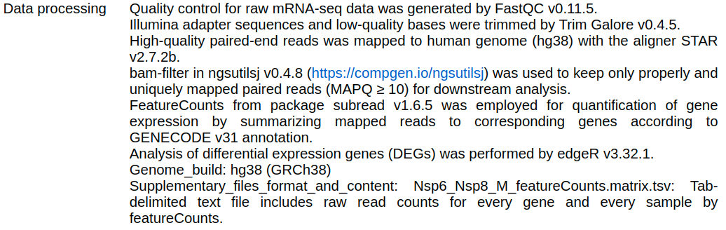
Today’s Data

• Data obtained from Gene Expression Omnibus GSE171742
• Stem cell derived cardiomyocytes with 4 treatment groups (Liu et al. 2023)
• All transfected using lentiviral vectors

1. Control
2. Nsp6 over-expression
3. Nsp8 over-expression
4. M over-expression

Today’s Data

Today’s Data

• Well documented metadata! 🤓
• We know exact versions of all tools and annotations

Loading Packages

library(tidyverse)
library(magrittr)
library(edgeR)
library(AnnotationHub)
library(rtracklayer)
library(plyranges)
library(patchwork)
library(scales)
library(glue)
library(ggrepel)
library(pheatmap)
library(parallel)
theme_set(theme_bw())

Getting Annotations

• Which one shall we choose?

ah <- AnnotationHub()
ah %>% subset(dataprovider == "Gencode" & genome == "GRCh38") %>% query("v31")

AnnotationHub with 9 records
# snapshotDate(): 2024-04-30
# $dataprovider: Gencode
# $species: Homo sapiens
# $rdataclass: GRanges
# additional mcols(): taxonomyid, genome, description,
#   coordinate_1_based, maintainer, rdatadateadded, preparerclass, tags,
#   rdatapath, sourceurl, sourcetype 
# retrieve records with, e.g., 'object[["AH75118"]]' 

            title                                                    
  AH75118 | gencode.v31.2wayconspseudos.gff3.gz                      
  AH75119 | gencode.v31.annotation.gff3.gz                           
  AH75120 | gencode.v31.basic.annotation.gff3.gz                     
  AH75121 | gencode.v31.chr_patch_hapl_scaff.annotation.gff3.gz      
  AH75122 | gencode.v31.chr_patch_hapl_scaff.basic.annotation.gff3.gz
  AH75123 | gencode.v31.long_noncoding_RNAs.gff3.gz                  
  AH75124 | gencode.v31.polyAs.gff3.gz                               
  AH75125 | gencode.v31.primary_assembly.annotation.gff3.gz          
  AH75126 | gencode.v31.tRNAs.gff3.gz                                

Getting Annotations

gtf <- ah[["AH75121"]] # This will take several minutes
genes <- gtf %>% 
  filter(type == "gene") %>% 
  select(starts_with("gene"))
genes

GRanges object with 66738 ranges and 3 metadata columns:
            seqnames        ranges strand |           gene_id              gene_type   gene_name
               <Rle>     <IRanges>  <Rle> |       <character>            <character> <character>
      [1]       chr1   11869-14409      + | ENSG00000223972.5 transcribed_unproces..     DDX11L1
      [2]       chr1   14404-29570      - | ENSG00000227232.5 unprocessed_pseudogene      WASH7P
      [3]       chr1   17369-17436      - | ENSG00000278267.1                  miRNA   MIR6859-1
      [4]       chr1   29554-31109      + | ENSG00000243485.5                 lncRNA MIR1302-2HG
      [5]       chr1   30366-30503      + | ENSG00000284332.1                  miRNA   MIR1302-2
      ...        ...           ...    ... .               ...                    ...         ...
  [66734] KI270734.1   72411-74814      + | ENSG00000276017.1         protein_coding  AC007325.1
  [66735] KI270734.1 131494-137392      + | ENSG00000278817.1         protein_coding  AC007325.4
  [66736] KI270734.1 138082-161852      - | ENSG00000277196.4         protein_coding  AC007325.2
  [66737] KI270744.1   51009-51114      - | ENSG00000278625.1                  snRNA     RF00026
  [66738] KI270750.1 148668-148843      + | ENSG00000277374.1                  snRNA     RF00003
  -------
  seqinfo: 407 sequences from an unspecified genome; no seqlengths

Getting Gene Lengths

• The simplest way is to add the width of all exonic regions

gene_lengths <- gtf %>% 
  filter(type == "exon") %>% 
  split(.$gene_id) %>% 
  reduce() %>% 
  width() %>% 
  mclapply(sum, mc.cores = 4) %>% 
  unlist()
genes$length <- gene_lengths[genes$gene_id]

Loading Counts

• Data is exactly as produced by featureCounts (Liao, Smyth, and Shi 2014)
  • Tab-delimited but with some weird columns
• Let’s have a sneak preview

read_tsv("data/GSE171742_counts.out.gz", n_max = 6)

# A tibble: 6 × 18
  Geneid      Chr   Start End   Strand Length `1_control` `6_control` `11_control` `2_Nsp6` `7_Nsp6`
  <chr>       <chr> <chr> <chr> <chr>   <dbl>       <dbl>       <dbl>        <dbl>    <dbl>    <dbl>
1 ENSG000000… chrX… 1006… 1006… -;-;-…   4535        5211        6192         4542     4328     5283
2 ENSG000000… chrX… 1005… 1005… +;+;+…   1476          65         178           96       50       86
3 ENSG000000… chr2… 5093… 5093… -;-;-…   1207        1454        1889         1329     1472     1684
4 ENSG000000… chr1… 1698… 1698… -;-;-…   6883         628         548          522      560      636
5 ENSG000000… chr1… 1696… 1696… +;+;+…   5970         191         241          150      146      254
6 ENSG000000… chr1… 2761… 2761… -;-;-…   3382           0           0            0        0        0
# ℹ 7 more variables: `12_Nsp6` <dbl>, `3_Nsp8` <dbl>, `8_Nsp8` <dbl>, `13_Nsp8` <dbl>,
#   `4_M` <dbl>, `9_M` <dbl>, `14_M` <dbl>

Which columns do we need? How would you parse them?

Loading Counts

• The best form for counts is as a matrix

counts <- read_tsv("data/GSE171742_counts.out.gz") %>% 
  dplyr::select(Geneid, contains("_")) %>% 
  as.data.frame() %>% 
  column_to_rownames("Geneid") %>% 
  as.matrix()
glimpse(counts)

 num [1:66738, 1:12] 5211 65 1454 628 191 ...
 - attr(*, "dimnames")=List of 2
  ..$ : chr [1:66738] "ENSG00000000003.14" "ENSG00000000005.6" "ENSG00000000419.12" "ENSG00000000457.14" ...
  ..$ : chr [1:12] "1_control" "6_control" "11_control" "2_Nsp6" ...

Checking Annotations

• Compare these with the annotations we have

setdiff(rownames(counts), genes$gene_id)

 [1] "ENSG00000002586.20_PAR_Y" "ENSG00000124333.16_PAR_Y" "ENSG00000124334.17_PAR_Y"
 [4] "ENSG00000167393.17_PAR_Y" "ENSG00000168939.11_PAR_Y" "ENSG00000169084.14_PAR_Y"
 [7] "ENSG00000169093.16_PAR_Y" "ENSG00000169100.14_PAR_Y" "ENSG00000178605.13_PAR_Y"
[10] "ENSG00000182162.11_PAR_Y" "ENSG00000182378.14_PAR_Y" "ENSG00000182484.15_PAR_Y"
[13] "ENSG00000185203.12_PAR_Y" "ENSG00000185291.11_PAR_Y" "ENSG00000185960.14_PAR_Y"
[16] "ENSG00000196433.13_PAR_Y" "ENSG00000197976.12_PAR_Y" "ENSG00000198223.16_PAR_Y"
[19] "ENSG00000205755.11_PAR_Y" "ENSG00000214717.12_PAR_Y" "ENSG00000223274.6_PAR_Y" 
[22] "ENSG00000223484.7_PAR_Y"  "ENSG00000223511.7_PAR_Y"  "ENSG00000223571.6_PAR_Y" 
[25] "ENSG00000223773.7_PAR_Y"  "ENSG00000225661.7_PAR_Y"  "ENSG00000226179.6_PAR_Y" 
[28] "ENSG00000227159.8_PAR_Y"  "ENSG00000228410.6_PAR_Y"  "ENSG00000228572.7_PAR_Y" 
[31] "ENSG00000229232.6_PAR_Y"  "ENSG00000230542.6_PAR_Y"  "ENSG00000234622.6_PAR_Y" 
[34] "ENSG00000234958.6_PAR_Y"  "ENSG00000236017.8_PAR_Y"  "ENSG00000236871.7_PAR_Y" 
[37] "ENSG00000237040.6_PAR_Y"  "ENSG00000237531.6_PAR_Y"  "ENSG00000237801.6_PAR_Y" 
[40] "ENSG00000265658.6_PAR_Y"  "ENSG00000270726.6_PAR_Y"  "ENSG00000275287.5_PAR_Y" 
[43] "ENSG00000277120.5_PAR_Y"  "ENSG00000280767.3_PAR_Y"  "ENSG00000281849.3_PAR_Y" 

• If we’re doing everything, we don’t need to check these
• Only for public data. Annotations can be difficult to untangle

• Should we remove the suffixes?

Checking Annotations

genes %>% subset(gene_id == "ENSG00000002586.20")

GRanges object with 2 ranges and 4 metadata columns:
      seqnames          ranges strand |            gene_id      gene_type   gene_name    length
         <Rle>       <IRanges>  <Rle> |        <character>    <character> <character> <integer>
  [1]     chrX 2691187-2741309      + | ENSG00000002586.20 protein_coding        CD99      9716
  [2]     chrY 2691187-2741309      + | ENSG00000002586.20 protein_coding        CD99      9716
  -------
  seqinfo: 407 sequences from an unspecified genome; no seqlengths

• How can we resolve this?

Checking Annotations

genes <- genes %>% 
  mutate(
    gene_id = case_when(
      duplicated(gene_id) ~ paste0(gene_id, "_PAR_Y"),
      TRUE ~ gene_id
    )
  ) 
subset(genes, duplicated(gene_id))

GRanges object with 0 ranges and 4 metadata columns:
   seqnames    ranges strand |     gene_id   gene_type   gene_name    length
      <Rle> <IRanges>  <Rle> | <character> <character> <character> <integer>
  -------
  seqinfo: 407 sequences from an unspecified genome; no seqlengths

DGE Analysis

Basic Workflow

1. Remove low-expressed & undetectable genes
2. Normalise the data
3. Estimate dispersions
4. Perform Statistical Tests
5. Enrichment Testing

• Careful checks at every step to inform decisions

DGEList Objects

• We’ll use edgeR for DGE analysis (Robinson, McCarthy, and Smyth 2010)
• Counts, sample metadata and gene annotations stored in a single S4 object
  • DGEList: Digital Gene Expression List
  • Gene & metadata elements need to be data.frame objects
  • Will be coerced if able . . .
• DESeq2 is a common alternative (Love, Huber, and Anders 2014)
• Uses an extension of SummarizedExperiment objects

• Both methods are gold-standard but neither perfect for every dataset
• Both Wolfgang Huber & Gordon Smyth are exceptional statisticians
• Will try get to DESeq2 later in the session

DGEList Objects

• How can we get sample metadata?

samples <- tibble(id = colnames(counts)) %>% 
  separate(id, into = c("replicate", "treatment"), remove = FALSE) %>% 
  mutate(
    treatment = as.factor(treatment),
    group = as.integer(treatment)
  )
samples

# A tibble: 12 × 4
   id         replicate treatment group
   <chr>      <chr>     <fct>     <int>
 1 1_control  1         control       1
 2 6_control  6         control       1
 3 11_control 11        control       1
 4 2_Nsp6     2         Nsp6          3
 5 7_Nsp6     7         Nsp6          3
 6 12_Nsp6    12        Nsp6          3
 7 3_Nsp8     3         Nsp8          4
 8 8_Nsp8     8         Nsp8          4
 9 13_Nsp8    13        Nsp8          4
10 4_M        4         M             2
11 9_M        9         M             2
12 14_M       14        M             2

Will be in the same order as counts

DGEList Objects

• Annotations appear to match the counts
  • Counts for 66,738 genes
  • Annotations for 66,738 genes
• But will be in a different order
  • Counts in order of name
  • Annotations in genomic order

DGEList Objects

genes %>% setNames(.$gene_id) %>% .[rownames(counts)]

GRanges object with 66738 ranges and 4 metadata columns:
                     seqnames              ranges strand |            gene_id      gene_type
                        <Rle>           <IRanges>  <Rle> |        <character>    <character>
  ENSG00000000003.14     chrX 100627109-100639991      - | ENSG00000000003.14 protein_coding
   ENSG00000000005.6     chrX 100584936-100599885      + |  ENSG00000000005.6 protein_coding
  ENSG00000000419.12    chr20   50934867-50958555      - | ENSG00000000419.12 protein_coding
  ENSG00000000457.14     chr1 169849631-169894267      - | ENSG00000000457.14 protein_coding
  ENSG00000000460.17     chr1 169662007-169854080      + | ENSG00000000460.17 protein_coding
                 ...      ...                 ...    ... .                ...            ...
   ENSG00000288107.1    chr10 133565797-133629507      + |  ENSG00000288107.1         lncRNA
   ENSG00000288108.1     chr5     1931058-1933985      - |  ENSG00000288108.1         lncRNA
   ENSG00000288109.1    chr17   67658015-67659465      - |  ENSG00000288109.1         lncRNA
   ENSG00000288110.1     chr8     4496392-4503392      + |  ENSG00000288110.1         lncRNA
   ENSG00000288111.1     chr3 130181346-130188814      + |  ENSG00000288111.1         lncRNA
                       gene_name    length
                     <character> <integer>
  ENSG00000000003.14      TSPAN6      4535
   ENSG00000000005.6        TNMD      1476
  ENSG00000000419.12        DPM1      1207
  ENSG00000000457.14       SCYL3      6883
  ENSG00000000460.17    C1orf112      5970
                 ...         ...       ...
   ENSG00000288107.1  AL731769.2      5662
   ENSG00000288108.1  AC126768.3       509
   ENSG00000288109.1  AC079331.3       748
   ENSG00000288110.1  AC010941.1      2417
   ENSG00000288111.1  AC130888.1       454
  -------
  seqinfo: 407 sequences from an unspecified genome; no seqlengths

DGEList Objects

dge <- DGEList(
  counts = counts,
  samples = tibble(id = colnames(counts)) %>% left_join(samples),
  genes = genes %>% 
    setNames(.$gene_id) %>% 
    .[rownames(counts)] %>% 
    as.data.frame(row.names = names(.))
)
dge

An object of class "DGEList"
$counts
                   1_control 6_control 11_control 2_Nsp6 7_Nsp6 12_Nsp6 3_Nsp8 8_Nsp8 13_Nsp8  4_M
ENSG00000000003.14      5211      6192       4542   4328   5283    4336   4330   5208    4635 4743
ENSG00000000005.6         65       178         96     50     86      83     67     92      80   51
ENSG00000000419.12      1454      1889       1329   1472   1684    1368   1666   2042    1707 1822
ENSG00000000457.14       628       548        522    560    636     492    530    500     498  622
ENSG00000000460.17       191       241        150    146    254     164    161    179     183  173
                    9_M 14_M
ENSG00000000003.14 5498 5172
ENSG00000000005.6    70   64
ENSG00000000419.12 2293 1987
ENSG00000000457.14  513  560
ENSG00000000460.17  256  228
66733 more rows ...

$samples
           group lib.size norm.factors         id replicate treatment
1_control      1 38633196            1  1_control         1   control
6_control      1 48184412            1  6_control         6   control
11_control     1 34566631            1 11_control        11   control
2_Nsp6         3 33088151            1     2_Nsp6         2      Nsp6
7_Nsp6         3 41621703            1     7_Nsp6         7      Nsp6
7 more rows ...

$genes
                   seqnames     start       end  width strand            gene_id      gene_type
ENSG00000000003.14     chrX 100627109 100639991  12883      - ENSG00000000003.14 protein_coding
ENSG00000000005.6      chrX 100584936 100599885  14950      +  ENSG00000000005.6 protein_coding
ENSG00000000419.12    chr20  50934867  50958555  23689      - ENSG00000000419.12 protein_coding
ENSG00000000457.14     chr1 169849631 169894267  44637      - ENSG00000000457.14 protein_coding
ENSG00000000460.17     chr1 169662007 169854080 192074      + ENSG00000000460.17 protein_coding
                   gene_name length
ENSG00000000003.14    TSPAN6   4535
ENSG00000000005.6       TNMD   1476
ENSG00000000419.12      DPM1   1207
ENSG00000000457.14     SCYL3   6883
ENSG00000000460.17  C1orf112   5970
66733 more rows ...

DGEList Objects

• Key elements have different but related dimensions

dim(dge)

[1] 66738    12

dim(dge$counts)

[1] 66738    12

dim(dge$samples)

[1] 12  6

dim(dge$genes)

[1] 66738     9

• samples is column metadata \(\implies\) genes is row metadata

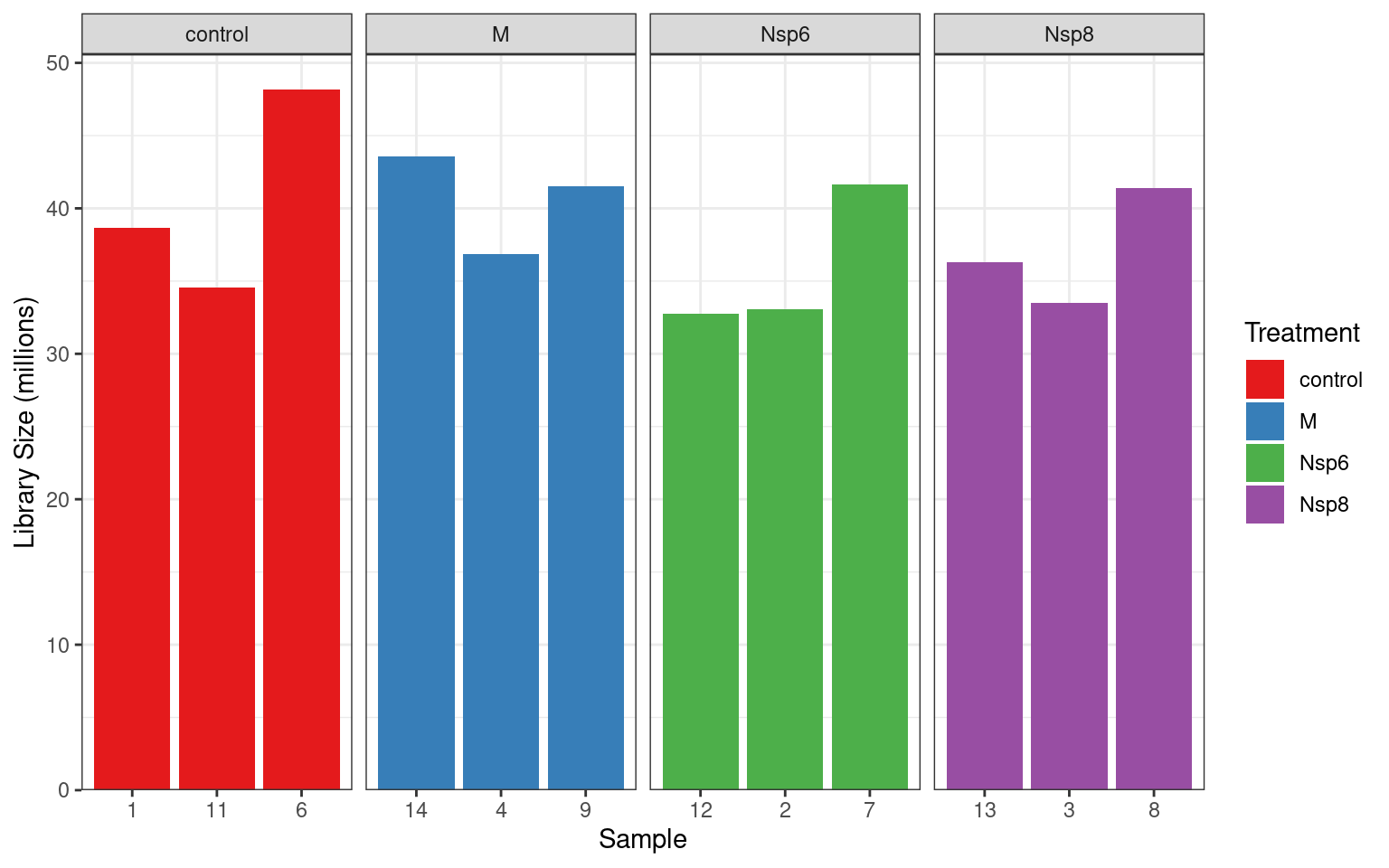
Library Sizes

• The very first step with counts \(\implies\) library sizes
• This is the total number of reads (i.e. RNA fragments) assigned to genes
• Ideally >20m reads per sample
• Those below 10m reads are generally considered as problematic
  • Context dependent

Library Sizes

dge$samples %>% 
  ggplot(aes(replicate, lib.size / 1e6, fill = treatment)) +
  geom_col() +
  facet_wrap(~treatment, nrow = 1, scales = "free_x") +
  labs(x = "Sample", y = "Library Size (millions)", fill = "Treatment") +
  scale_y_continuous(expand = expansion(c(0, 0.05))) +
  scale_fill_brewer(palette = "Set1")

Click to show figure

Library Sizes

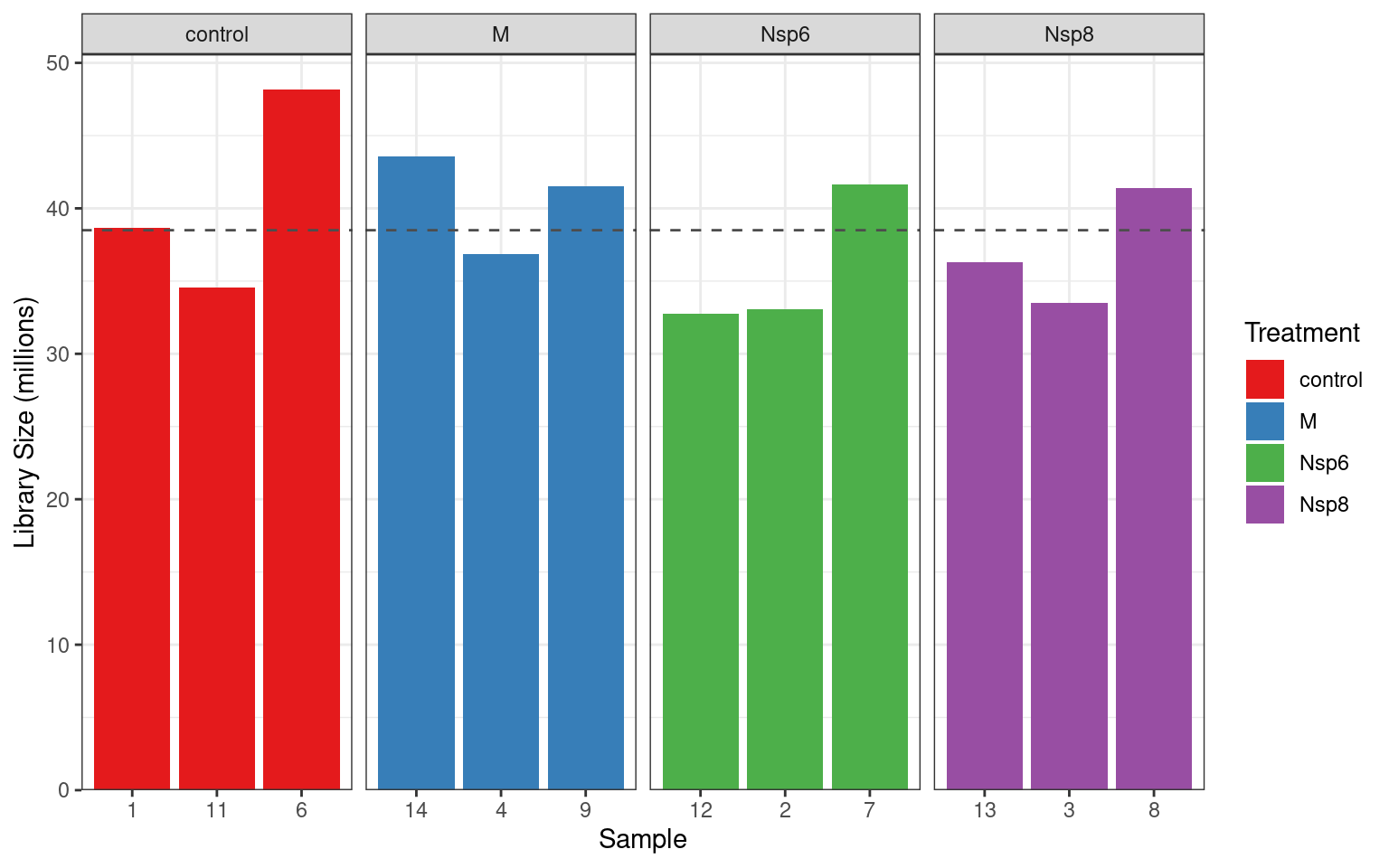
• We can get fancy and add the mean value

dge$samples %>% 
  ggplot(aes(replicate, lib.size / 1e6, fill = treatment)) +
  geom_col() +
  geom_hline(
    aes(yintercept = lib.size),
    data = . %>% summarise(lib.size = mean(lib.size / 1e6)),
    linetype = 2, colour = "grey30"
  ) +
  facet_wrap(~treatment, nrow = 1, scales = "free_x") +
  labs(x = "Sample", y = "Library Size (millions)", fill = "Treatment") +
  scale_y_continuous(expand = expansion(c(0, 0.05))) +
  scale_fill_brewer(palette = "Set1")

Click to show figure

These look like really good libraries so far

Detected Vs Undetected Genes

• By adding counts across samples and seeing how many are zero
  \(\implies\) non-detectable genes

dge$counts %>% 
  rowSums() %>% 
  equals(0) %>% 
  sum()

[1] 27211

• Genes with low counts can also be removed
  • These end up being highly variable
  • Uninformative statistically

Detected Vs Undetected Genes

• No set method for considering a gene as too low to bother with
• Can use raw counts below some value
• Counts within a group above some value \(\implies\) detected within a treatment

• Counts per million reads (CPM) is a common measure used in abundance analysis
• Take the library sizes / 1e6 & divide counts by this value \(\implies\) CPM
• Can also use logCPM
  • Adds a non-zero value to every gene to avoid zeroes

Detected Vs Undetected Genes

• edgeR provides a function filterByExpr()
• Flags genes for removal or discarding based on counts
• Set minimum CPM as min.count \(\times 1e6\) / median(lib.size)
• Set minimum total counts

• Genes are retained if CPM > minCPM in \(\geq n\) samples
  • \(n\) is the smallest treatment group
• Default settings may be a little generous for this dataset

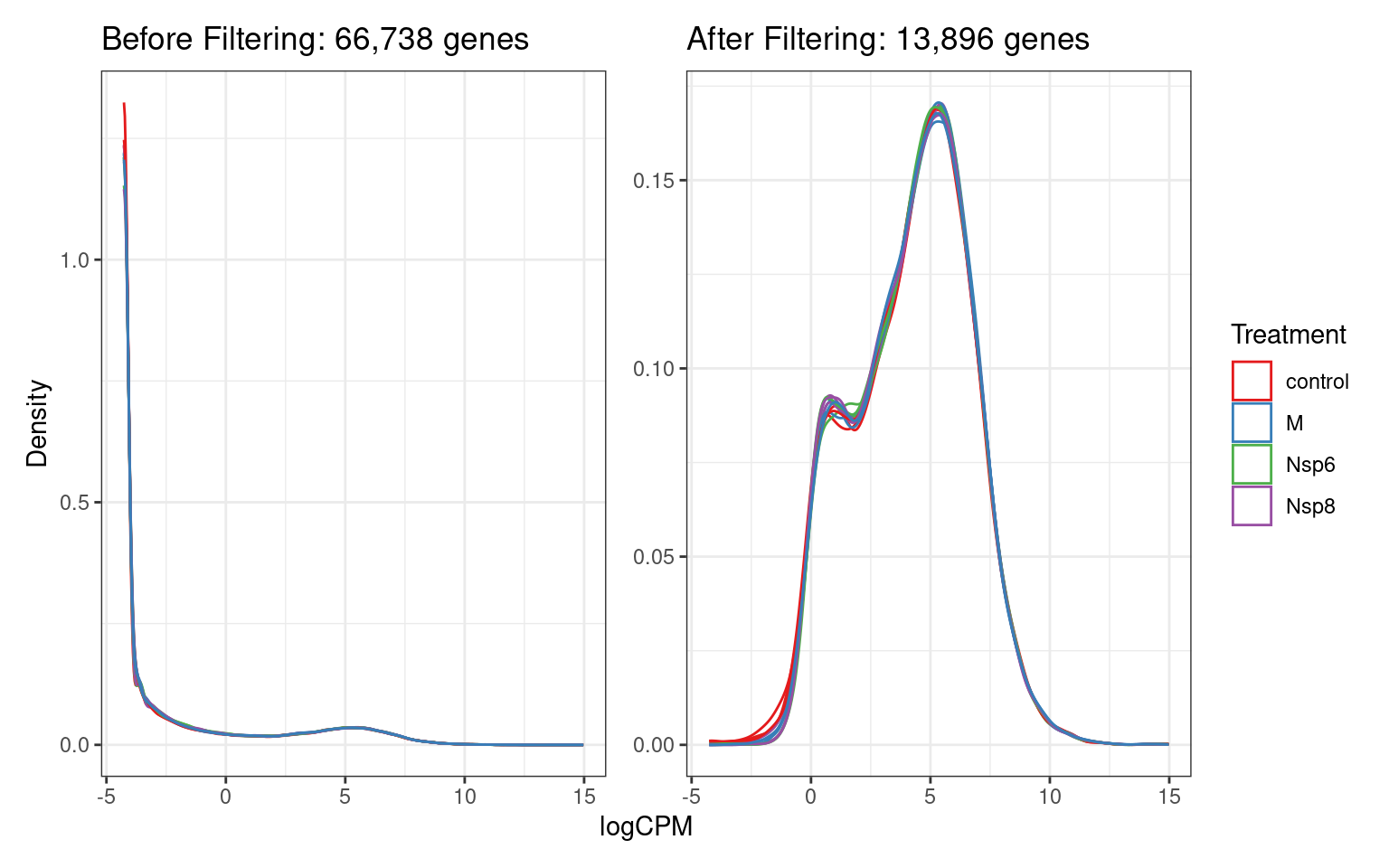
Detected Vs Undetected Genes

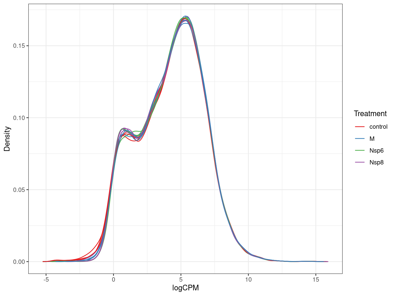
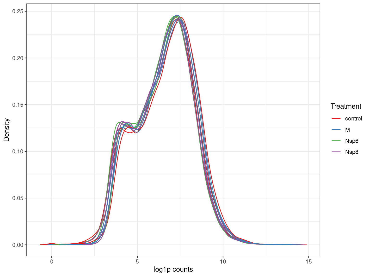
• If we require > 1CPM in at least 3 samples

min_count <- dge$samples$lib.size %>% 
  median() %>% 
  divide_by(1e6) %>% 
  round(0)
min_count

[1] 38

min_total <- 150
keep <- filterByExpr(dge, min.count = min_count, min.total.count = 150)

Detected Vs Undetected Genes

A <- dge$counts %>% 
  cpm(log = TRUE) %>% 
  as_tibble(rownames = "gene_id") %>% 
  pivot_longer(-all_of("gene_id"), names_to = "id", values_to = "logCPM") %>% 
  left_join(dge$samples) %>% 
  ggplot(aes(logCPM, after_stat(density), group = id)) +
  geom_density(aes(colour = treatment)) +
  ggtitle(glue("Before Filtering: {comma(length(keep))} genes")) +
  labs(y = "Density", colour = "Treatment") +
  scale_colour_brewer(palette = "Set1")
B <- dge$counts[keep,] %>% 
  cpm(log = TRUE) %>% 
  as_tibble(rownames = "gene_id") %>% 
  pivot_longer(-all_of("gene_id"), names_to = "id", values_to = "logCPM") %>% 
  left_join(dge$samples) %>% 
  ggplot(aes(logCPM, after_stat(density), group = id)) +
  geom_density(aes(colour = treatment)) +
  ggtitle(glue("After Filtering: {comma(sum(keep))} genes")) +
  labs(y = "Density", colour = "Treatment") +
  scale_colour_brewer(palette = "Set1")
A + B + plot_layout(guides = "collect", axes = "collect")

Click to show figure

Detected Vs Undetected Genes

• Create new object once satisfied with the filtering strategy
• Passing the logical vector will subset counts & genes correctly
  • The original library sizes are retained

dge_filter <- dge[keep,]
dge_filter

An object of class "DGEList"
$counts
                   1_control 6_control 11_control 2_Nsp6 7_Nsp6 12_Nsp6 3_Nsp8 8_Nsp8 13_Nsp8  4_M
ENSG00000000003.14      5211      6192       4542   4328   5283    4336   4330   5208    4635 4743
ENSG00000000005.6         65       178         96     50     86      83     67     92      80   51
ENSG00000000419.12      1454      1889       1329   1472   1684    1368   1666   2042    1707 1822
ENSG00000000457.14       628       548        522    560    636     492    530    500     498  622
ENSG00000000460.17       191       241        150    146    254     164    161    179     183  173
                    9_M 14_M
ENSG00000000003.14 5498 5172
ENSG00000000005.6    70   64
ENSG00000000419.12 2293 1987
ENSG00000000457.14  513  560
ENSG00000000460.17  256  228
13891 more rows ...

$samples
           group lib.size norm.factors         id replicate treatment
1_control      1 38633196            1  1_control         1   control
6_control      1 48184412            1  6_control         6   control
11_control     1 34566631            1 11_control        11   control
2_Nsp6         3 33088151            1     2_Nsp6         2      Nsp6
7_Nsp6         3 41621703            1     7_Nsp6         7      Nsp6
7 more rows ...

$genes
                   seqnames     start       end  width strand            gene_id      gene_type
ENSG00000000003.14     chrX 100627109 100639991  12883      - ENSG00000000003.14 protein_coding
ENSG00000000005.6      chrX 100584936 100599885  14950      +  ENSG00000000005.6 protein_coding
ENSG00000000419.12    chr20  50934867  50958555  23689      - ENSG00000000419.12 protein_coding
ENSG00000000457.14     chr1 169849631 169894267  44637      - ENSG00000000457.14 protein_coding
ENSG00000000460.17     chr1 169662007 169854080 192074      + ENSG00000000460.17 protein_coding
                   gene_name length
ENSG00000000003.14    TSPAN6   4535
ENSG00000000005.6       TNMD   1476
ENSG00000000419.12      DPM1   1207
ENSG00000000457.14     SCYL3   6883
ENSG00000000460.17  C1orf112   5970
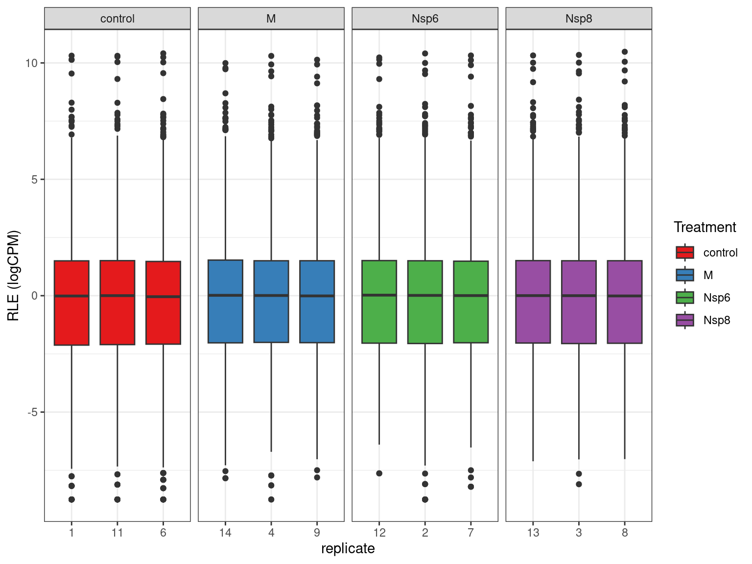
13891 more rows ...

Normalisation

• Normalisation is a very common step in transcriptomic analysis
• Helps to account for differences in library composition
  • e.g. are some libraries dominated by a handful of highly abundant genes
• The default in edgeR is TMM (Robinson and Oshlack 2010)
• DESeq2 uses RLE normalisation
  • Very similar in principle

Statistical Analysis of Counts

• Poisson models number of events per unit
  • e.g. telephone calls per minute
• The rate parameter (\(\lambda\)) models this
• mean occurrence = average rate = \(\lambda\)
• Variance is fixed at \(\lambda\)
  • If variance \(\neq \lambda \implies\) not Poisson data

• The basic model for edgeR is a Negative Binomial Model
  • NB: mean = \(\lambda\); variance = \(\lambda + r\)
• Multiple strategies for obtaining estimates

Statistical Analysis of Counts

• Counts / gene (i.e. \(y_{gi}\)) are a function of library size (\(L_i\))
• Gene length is fixed across samples \(\implies\) library size is not
• Dividing by library size is a way of normalising counts

\[ \log (y_{gi} / L_i) = \beta_0 + \beta_1 + ... \]

Normalisation

• Calculation of normalisation factors (\(Y_i\)) per sample
  • The idealised normalisation factor is \(Y_i = 1\)
• Can use scaled library sizes \(L^*_i = Y_i \times L_i\)

\[ \log (y_{gi} / L^*_i) = \beta_0 + \beta_1 + ... \]

TMM Normalisation

dge_filter <- calcNormFactors(dge_filter)
dge_filter$samples

           group lib.size norm.factors         id replicate treatment
1_control      1 38633196    0.9943180  1_control         1   control
6_control      1 48184412    0.9770121  6_control         6   control
11_control     1 34566631    0.9883140 11_control        11   control
2_Nsp6         3 33088151    1.0157571     2_Nsp6         2      Nsp6
7_Nsp6         3 41621703    0.9963827     7_Nsp6         7      Nsp6
12_Nsp6        3 32724713    1.0060007    12_Nsp6        12      Nsp6
3_Nsp8         4 33502022    1.0076816     3_Nsp8         3      Nsp8
8_Nsp8         4 41364663    0.9977052     8_Nsp8         8      Nsp8
13_Nsp8        4 36288023    1.0027832    13_Nsp8        13      Nsp8
4_M            2 36851725    1.0081808        4_M         4         M
9_M            2 41546877    0.9987653        9_M         9         M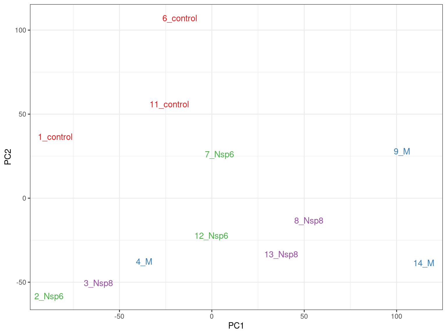
14_M           2 43587502    1.0076991       14_M        14         M

• The clustering around 1 suggests very similar libraries

PCA Analysis

• edgeR offers plotMDS() for quick exploration

plotMDS(
  dge_filter, 
  col = as.integer(dge_filter$samples$treatment)
)

• Takes top 500 most variable genes
• Uses base graphics

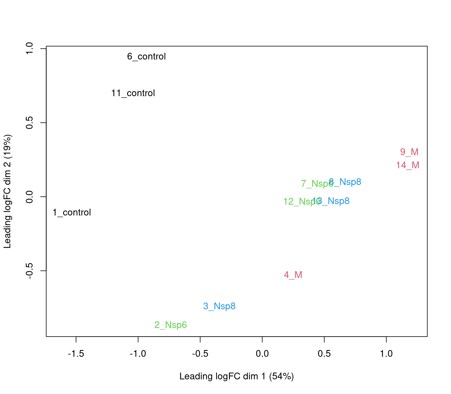
PCA Analysis

• logCPM values are very useful for PCA
  • Will now be calculated using the normalisation factors

pca <- dge_filter %>% 
  cpm(log = TRUE) %>% 
  t() %>% 
  prcomp(center = TRUE, scale. = TRUE)
summary(pca)

Importance of components:
                           PC1     PC2     PC3     PC4     PC5      PC6      PC7      PC8      PC9
Standard deviation     66.6493 50.4749 45.2310 31.7401 29.3998 25.88752 24.74707 21.51801 20.94233
Proportion of Variance  0.3197  0.1833  0.1472  0.0725  0.0622  0.04823  0.04407  0.03332  0.03156
Cumulative Proportion   0.3197  0.5030  0.6502  0.7227  0.7849  0.83316  0.87723  0.91056  0.94212
                           PC10     PC11      PC12
Standard deviation     20.27916 19.82675 2.753e-13
Proportion of Variance  0.02959  0.02829 0.000e+00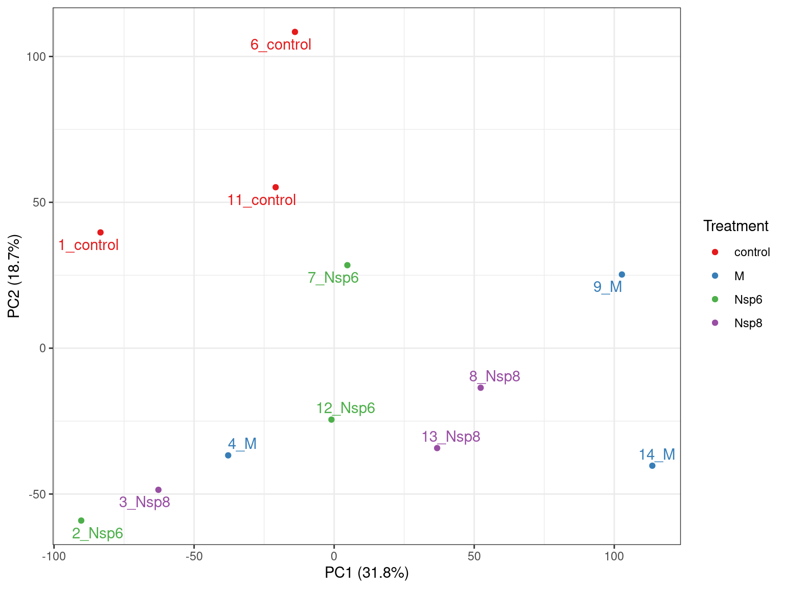
Cumulative Proportion   0.97171  1.00000 1.000e+00

prop_var <- summary(pca)$importance["Proportion of Variance",]

PCA Analysis

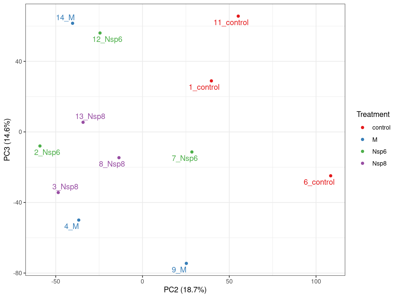
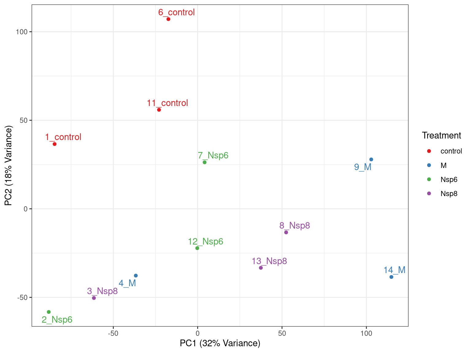
• PC1 vs PC2 shown below \(\implies\) easily modified to other components

• Simple PCA
• Enhanced Axis Labels

pca %>% 
  broom::tidy() %>% 
  pivot_wider(names_from = "PC", names_prefix = "PC", values_from = "value") %>% 
  dplyr::rename(id = row) %>% 
  left_join(dge_filter$samples) %>% 
  ggplot(aes(PC1, PC2, colour = treatment)) +
  geom_text(aes(label = id), show.legend = FALSE) +
  scale_colour_brewer(palette = "Set1")

Click to show figure

pca %>% 
  broom::tidy() %>% 
  pivot_wider(names_from = "PC", names_prefix = "PC", values_from = "value") %>% 
  dplyr::rename(id = row) %>% 
  left_join(dge_filter$samples) %>% 
  ggplot(aes(PC1, PC2, colour = treatment)) +
  geom_point() +
  geom_text_repel(aes(label = id), show.legend = FALSE) +
  labs(
    x = glue("PC1 ({percent(prop_var['PC1'])} Variance)"),
    y = glue("PC2 ({percent(prop_var['PC2'])} Variance)"),
    colour = "Treatment"
  ) +
  scale_colour_brewer(palette = "Set1")

Click to show figure

PCA Analysis

• What do we think the above is telling us?
• Does it look like treatment is contributing to the variance?
• Are there any other potential sources of variability?

• Looks to me like samples 2-4 had transfection issues
• Need to discuss with wet lab folks

The Design Matrix

• Before proceeding need to define a design matrix

X <- model.matrix(~treatment, dge_filter$samples)
X

           (Intercept) treatmentM treatmentNsp6 treatmentNsp8
1_control            1          0             0             0
6_control            1          0             0             0
11_control           1          0             0             0
2_Nsp6               1          0             1             0
7_Nsp6               1          0             1             0
12_Nsp6              1          0             1             0
3_Nsp8               1          0             0             1
8_Nsp8               1          0             0             1
13_Nsp8              1          0             0             1
4_M                  1          1             0             0
9_M                  1          1             0             0
14_M                 1          1             0             0
attr(,"assign")
[1] 0 1 1 1
attr(,"contrasts")
attr(,"contrasts")$treatment
[1] "contr.treatment"

The Design Matrix

• The first column will estimate average expression in control samples
• Remaining columns estimate the difference due to treatments
• (Almost) always modelled on the log2 scale \(\implies\) logFC

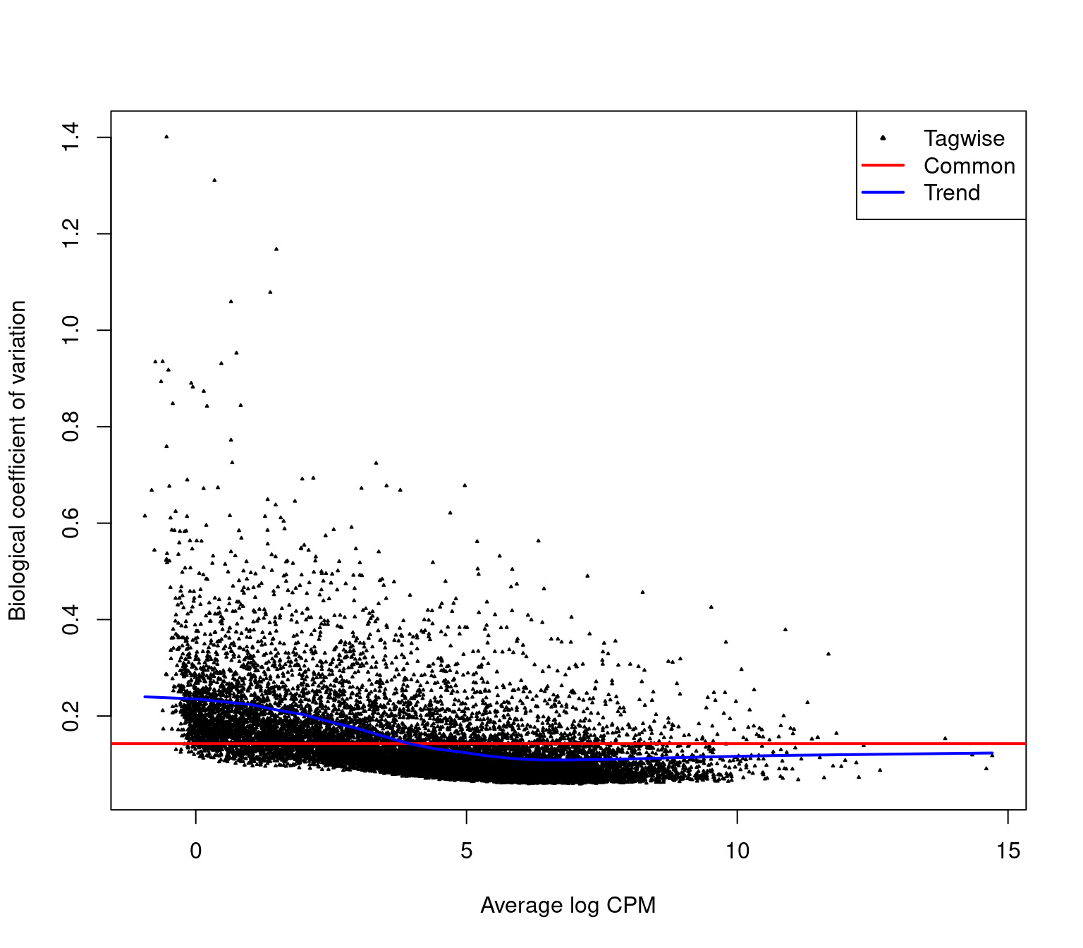
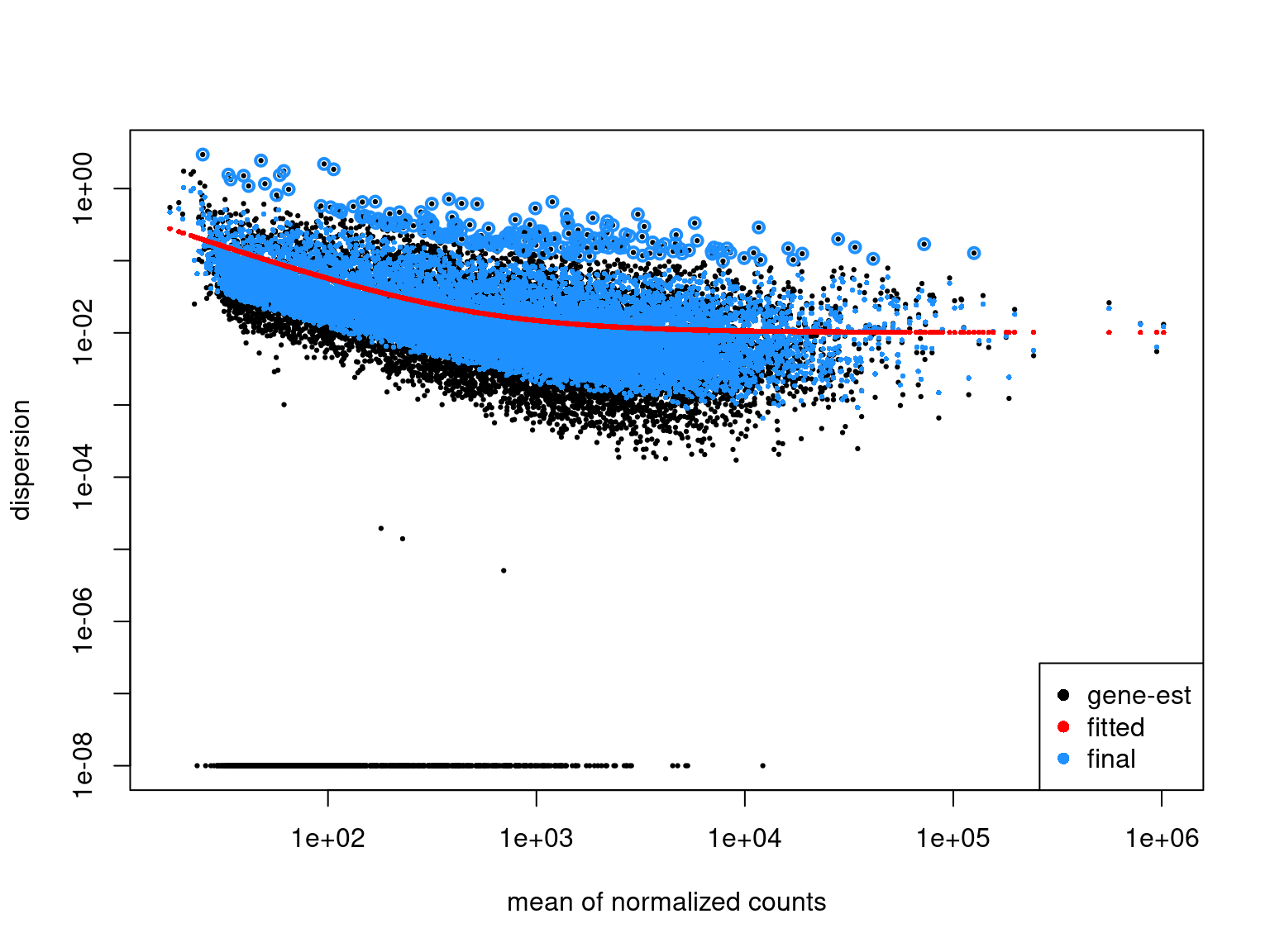
Estimating Dispersions

• We can estimate the dispersion parameter across the entire dataset
• edgeR models consider technical noise as Poisson with biological noise as over-dispersion
• This adds multiple elements to the DGEList
  • Essential for edgeR models
• Initial estimates are moderated using a global trend during model fitting

dge_filter <- estimateDisp(dge_filter, design = X)

Estimating Dispersions

# Output uses base graphics no ggplot
plotBCV(dge_filter, pch = 2)

Model Fitting

• The recommended approach for edgeR is to use Quasi-Likelihood fits (Lund et al. 2012)
  • Allows flexibility in over-dispersion parameters
• First we fit the model \(\implies\) then perform testing
• Using our design matrix, we will fit the model for all coefficients in X
  • Perform tests within each co-efficient
  • We’ll use the ‘M’ treatment

fit <- glmQLFit(dge_filter, design = X)

Model Testing

• Statistical tests use quasi-likelihood F-tests
• Use moderate dispersions (Empirical Bayes)
• By default, the top10 genes are returned

fit %>% glmQLFTest(coef = "treatmentM") %>% topTags()

Coefficient:  treatmentM 
                   seqnames     start       end  width strand            gene_id      gene_type
ENSG00000065609.14     chr6  83552880  83709691 156812      - ENSG00000065609.14 protein_coding
ENSG00000133878.9      chr8  33591330  33600023   8694      -  ENSG00000133878.9 protein_coding
ENSG00000112837.17     chr6  84687351  84764598  77248      - ENSG00000112837.17 protein_coding
ENSG00000125730.16    chr19   6677704   6730562  52859      - ENSG00000125730.16 protein_coding
ENSG00000144810.16     chr3  99638475  99799226 160752      + ENSG00000144810.16 protein_coding
ENSG00000112562.18     chr6 168441151 168673445 232295      + ENSG00000112562.18 protein_coding
ENSG00000118137.9     chr11 116835751 116837950   2200      -  ENSG00000118137.9 protein_coding
ENSG00000101335.10    chr20  36541497  36551447   9951      + ENSG00000101335.10 protein_coding
ENSG00000156113.23    chr10  76869601  77638369 768769      - ENSG00000156113.23 protein_coding
ENSG00000165118.15     chr9  83938311  83956986  18676      - ENSG00000165118.15 protein_coding
                   gene_name length     logFC    logCPM         F       PValue          FDR
ENSG00000065609.14    SNAP91   6651 -4.298482 5.7855158 1244.7901 4.457146e-13 6.193650e-09
ENSG00000133878.9     DUSP26   1971 -6.406627 0.9996001  320.3749 8.859485e-11 6.155570e-07
ENSG00000112837.17     TBX18   8654  4.614608 1.3852329  463.1117 1.329742e-10 6.159367e-07
ENSG00000125730.16        C3   8328  7.404154 1.9905031  222.5631 7.853570e-10 2.728330e-06
ENSG00000144810.16    COL8A1   9408  1.897573 4.2552562  221.7729 7.221342e-09 2.006955e-05
ENSG00000112562.18     SMOC2   4032  2.975471 2.9960180  214.3021 8.720084e-09 2.019572e-05
ENSG00000118137.9      APOA1   1424 -1.909907 6.8931539  201.6088 1.216484e-08 2.414894e-05
ENSG00000101335.10      MYL9   2808  2.208139 9.0902053  192.7708 1.553354e-08 2.553771e-05
ENSG00000156113.23    KCNMA1  35644  2.906831 4.0355987  190.5689 1.653997e-08 2.553771e-05
ENSG00000165118.15   C9orf64   2754  5.728040 1.8379059  176.1002 2.011799e-08 2.556070e-05

Model Testing

• Can easily collect all genes into a manageable object

res_M <- fit %>% 
  glmQLFTest(coef = "treatmentM") %>%
  topTags(n = Inf) %>% 
  as.data.frame() %>% 
  as_tibble()
res_M

# A tibble: 13,896 × 14
   seqnames     start       end  width strand gene_id  gene_type gene_name length logFC logCPM     F
   <fct>        <int>     <int>  <int> <fct>  <chr>    <chr>     <chr>      <int> <dbl>  <dbl> <dbl>
 1 chr6      83552880  83709691 156812 -      ENSG000… protein_… SNAP91      6651 -4.30   5.79 1245.
 2 chr8      33591330  33600023   8694 -      ENSG000… protein_… DUSP26      1971 -6.41   1.00  320.
 3 chr6      84687351  84764598  77248 -      ENSG000… protein_… TBX18       8654  4.61   1.39  463.
 4 chr19      6677704   6730562  52859 -      ENSG000… protein_… C3          8328  7.40   1.99  223.
 5 chr3      99638475  99799226 160752 +      ENSG000… protein_… COL8A1      9408  1.90   4.26  222.
 6 chr6     168441151 168673445 232295 +      ENSG000… protein_… SMOC2       4032  2.98   3.00  214.
 7 chr11    116835751 116837950   2200 -      ENSG000… protein_… APOA1       1424 -1.91   6.89  202.
 8 chr20     36541497  36551447   9951 +      ENSG000… protein_… MYL9        2808  2.21   9.09  193.
 9 chr10     76869601  77638369 768769 -      ENSG000… protein_… KCNMA1     35644  2.91   4.04  191.
10 chr9      83938311  83956986  18676 -      ENSG000… protein_… C9orf64     2754  5.73   1.84  176.
# ℹ 13,886 more rows
# ℹ 2 more variables: PValue <dbl>, FDR <dbl>

Multiple Testing

• Under H₀: ~1 in 20 random p-values will be < 0.05
• With ~14,000 genes \(\implies\) about 700 expected
• These would be Type 1 errors \(\implies\) false positives
  • We say something is happening, when it’s just noise

• The False Discovery Rate (FDR) controls Type 1 errors at a given rate
  • Using \(\alpha = 0.05 \implies\) happy with 5% of results being errors
  • Always just an estimate

sum(res_M$FDR < 0.05)

[1] 1409

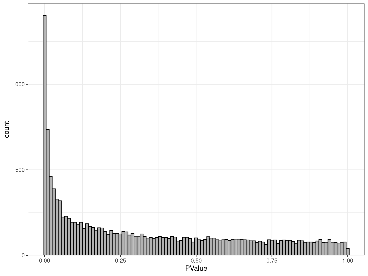
Inspection of P-values

• Under H₀ \(\implies\) \(p \sim \mathcal{U}(0, 1)\)
• Under H_A no distribution \(\implies\) peak near zero

res_M %>% 
  ggplot(aes(PValue)) +
  geom_histogram(binwidth = 0.01, fill = "grey70", colour = "black") +
  scale_y_continuous(expand = expansion(c(0, 0.05))) 

Click to show figure

Looks as expected

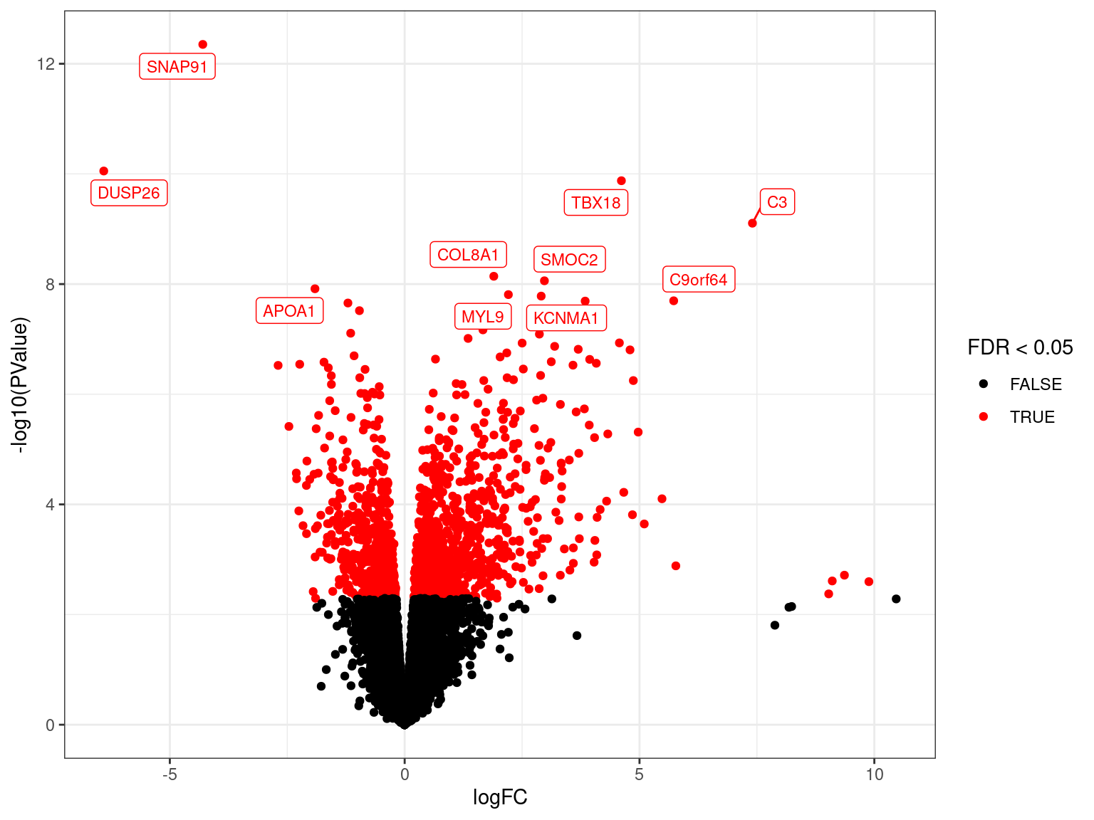
Volcano Plots

• Plot developed during microarray analysis
• Shows logFC against significance (\(p\)-values)

res_M %>% 
  ggplot(aes(logFC, -log10(PValue), colour = FDR < 0.05)) +
  geom_point() +
  geom_label_repel(
    aes(label = gene_name),
    data = . %>% 
      arrange(PValue) %>% 
      dplyr::slice(1:10),
    size = 3, show.legend = FALSE
  ) +
  scale_colour_manual(values = c("black", "red")) 

Click to show figure

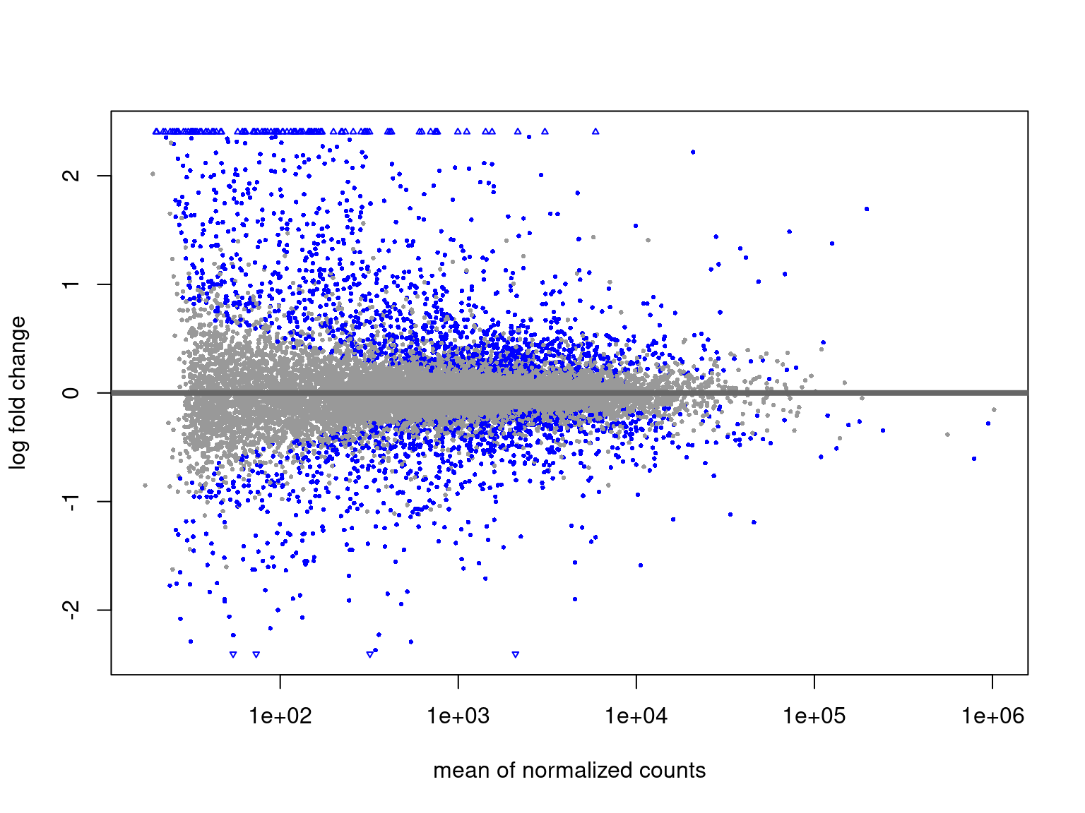
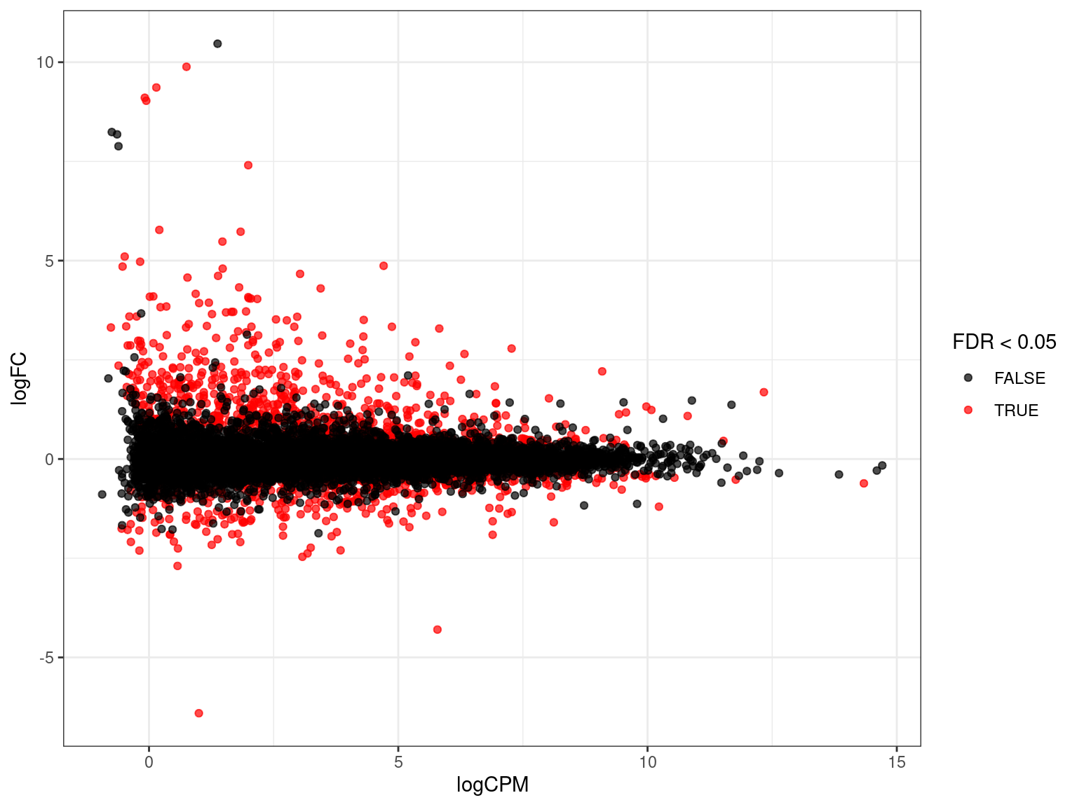
MA Plots

• Two-colour microarray data introduced MA plots
• Signal from two-colour arrays layered treat vs control in a single spot
  • A for intensity averages
  • M for mean intensity differences
• Still commonly used and the language remains
• Sometimes called MD (mean-difference) plots
  • edgeR provides plotMD()
• Show average expression on the x-axis and logFC on y-axis
  • How highly expressed are any DE genes?

MA Plots

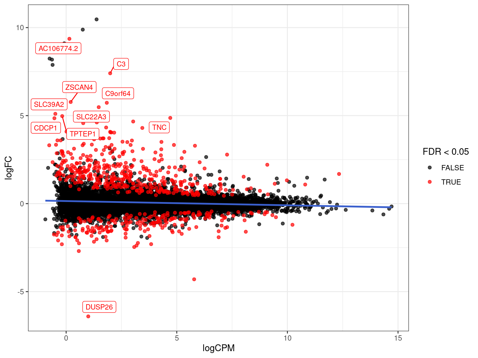
• Often start with an exploration then customise for our data

• Initial Plot
• Customised Plot

res_M %>% 
  ggplot(aes(logCPM, logFC)) +
  geom_point(aes(colour = FDR < 0.05), alpha = 0.7) +
  scale_colour_manual(values = c("black", "red"))

Click to show figure

res_M %>% 
  arrange(desc(PValue)) %>% # Why do this?
  ggplot(aes(logCPM, logFC, colour = FDR < 0.05)) +
  geom_point(alpha = 0.7) +
  geom_smooth(se = FALSE, colour = 'royalblue3', method = "lm") +
  geom_label_repel(
    aes(label = gene_name),
    data = . %>% 
      dplyr::filter(FDR < 0.05) %>% 
      arrange(desc(abs(logFC))) %>% 
      dplyr::slice(1:10),
    size = 3, show.legend = FALSE
  ) +
  scale_colour_manual(values = c("black", "red")) 

Click to show figure

Filtering of DE Genes

• There is a tendency of the most extreme logFC to be in low expressed genes
• The ratio of any number over a small number will \(\rightarrow \infty\)
• If there are “too many” DE genes \(\implies\) should we filter results?

• Early approaches were to filter on extreme logFC
• Biased results towards low-expressed genes

Range-Based Hypothesis Testing

• Traditional H₀ is \(\mu = 0\) against H_A \(\mu \neq 0\)
• An alternative is to use a range-based H₀ (McCarthy and Smyth 2009)
• Implemented in glmTreat()
• Default range is FC > 20% in either direction

res_treatM <- fit %>% 
  glmTreat(coef = "treatmentM", lfc = log2(1.2)) %>% 
  topTags(n = Inf) %>% 
  as.data.frame() %>% 
  as_tibble()
sum(res_treatM$FDR < 0.05)

[1] 596

Range-Based Hypothesis Testing

res_treatM %>% 
  arrange(desc(PValue)) %>% # Why do this?
  ggplot(aes(logCPM, logFC, colour = FDR < 0.05)) +
  geom_point(alpha = 0.7) +
  geom_smooth(se = FALSE, colour = 'royalblue3', method = "lm") +
  geom_label_repel(
    aes(label = gene_name),
    data = . %>% 
      dplyr::filter(FDR < 0.05) %>% 
      arrange(desc(abs(logFC))) %>% 
      dplyr::slice(1:10),
    size = 3, show.legend = FALSE
  ) +
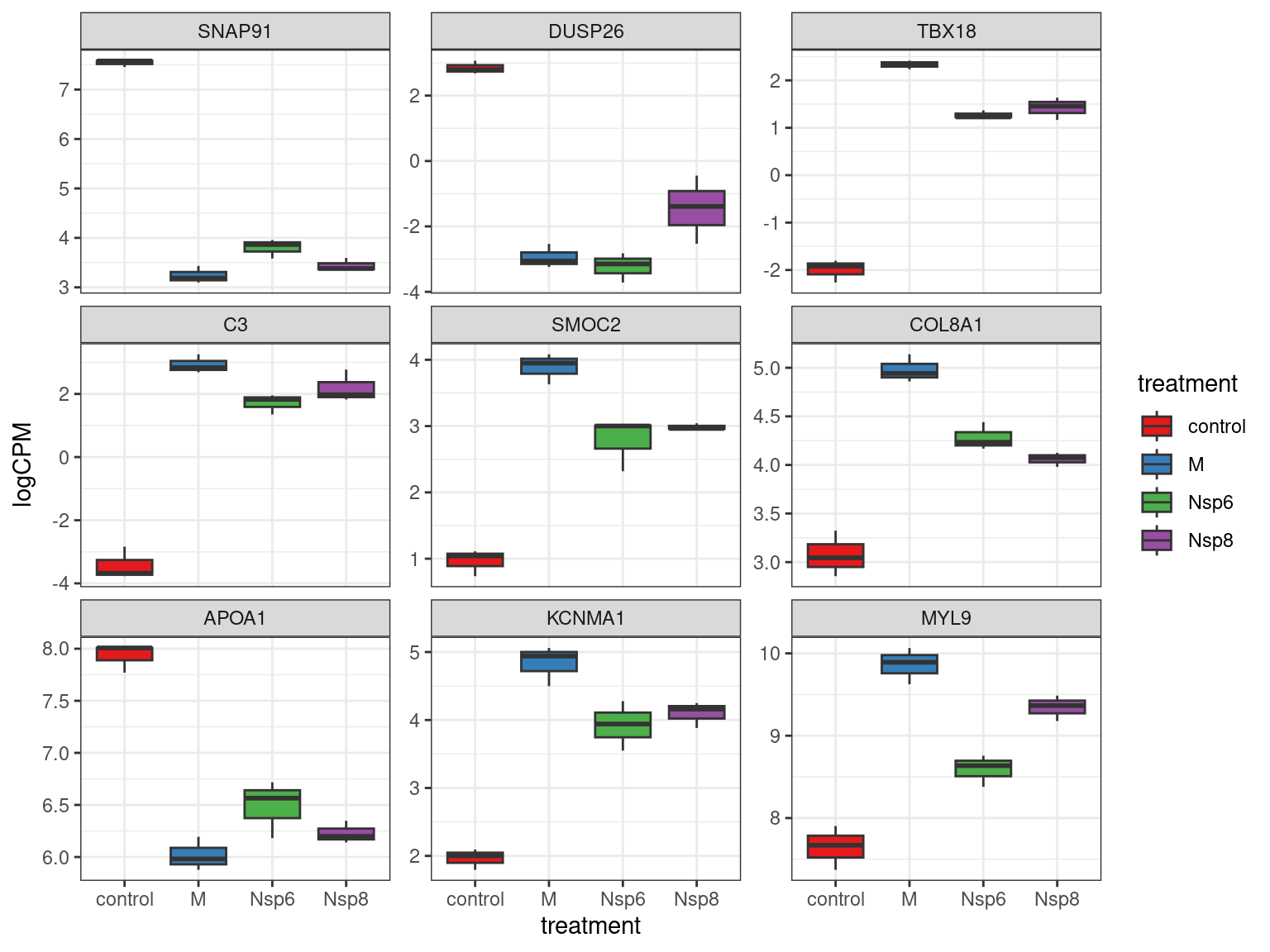
  scale_colour_manual(values = c("black", "red")) 

Click to show figure

Clearly some high logFC genes had weak statistical support

Checking Individual Genes

• Checking individual genes for changes in expression can be helpful
• Choosing a small number helps with interpretability

cpm(dge_filter, log = TRUE) %>% 
  .[res_treatM$gene_id[1:9],] %>% 
  as_tibble(rownames = "gene_id") %>% 
  pivot_longer(-all_of("gene_id"), names_to = "id", values_to = "logCPM") %>% 
  left_join(dge$genes) %>% 
  left_join(dge$samples) %>%
  mutate(gene_name = fct_inorder(gene_name)) %>% 
  ggplot(aes(treatment, logCPM, fill = treatment)) +
  geom_boxplot() +
  facet_wrap(~gene_name, scales = "free_y") +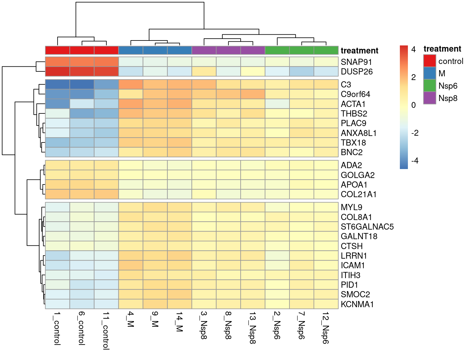
  scale_fill_brewer(palette = "Set1")

Click to show figure

Heatmaps Across Multiple Genes

• Showing larger groups of genes can also be informative
• Enables very basic clustering of genes

• The package pheatmap is a common resource
• Pre-dates the tidyverse \(\implies\) matrix and data.frame objects

Heatmaps Across Multiple Genes

1. Form a matrix from the top genes
2. Subtract the mean expression value
   • This retains variability but shows direction of change
3. Set rownames to be the gene-names

mat <- cpm(dge_filter, log = TRUE)[res_treatM$gene_id[1:25],] 
mat <- mat - rowMeans(mat)
rownames(mat) <- setNames(genes$gene_name, genes$gene_id)[rownames(mat)]

• Choosing too many genes can confuse rather than illustrate the results!!!

Heatmaps Across Multiple Genes

• Groups can be set using column annotations (annotation_col)
  • Requires a data.frame with rownames
• Group colours can also be passed as a list

pheatmap(
  mat, 
  annotation_col = samples %>%
    dplyr::select(id, treatment) %>% 
    as.data.frame() %>% 
    column_to_rownames("id"),
  annotation_colors = list(
    treatment = setNames(
      RColorBrewer::brewer.pal(4, "Set1"), levels(samples$treatment)
    )
  ),
  cutree_rows = 4
)

Click to show figure

Every column in the annotation df will be added as an annotation

Using DESeq2

DESeq2

• Another common package for RNASeq analysis is DESeq2 (Love, Huber, and Anders 2014)
• Uses S4 object more interconnected to other Bioconductor classes
• Different approach to dispersions
• Different statistical testing
• Feels a bit more like a “black-box” to me
  • More default settings for a similar workflow \(\implies\) fewer manual steps
• Is a very high-quality approach (as is edgeR)

DESeq2

library(DESeq2)
library(extraChIPs)
dds <- DESeqDataSetFromMatrix(
  dge_filter$counts, 
  colData = samples,
  rowData = dge_filter$genes %>% 
    makeGRangesFromDataFrame(keep.extra.columns = TRUE),
  design = ~ treatment
)
is(dds)

[1] "DESeqDataSet"               "RangedSummarizedExperiment" "SummarizedExperiment"      
[4] "RectangularData"            "Vector"                     "Annotated"                 
[7] "vector_OR_Vector"          

Summarized Experiment Objects

• SummarizedExperiment objects are a core Bioconductor class

getSlots("SummarizedExperiment")

            colData              assays               NAMES     elementMetadata            metadata 
        "DataFrame"    "Assays_OR_NULL" "character_OR_NULL"         "DataFrame"              "list" 

• Any number of assays can be added
  • Usually matrices with identical dimensions
• colData holds the sample-level metadata

Summarized Experiment Objects

• RangedSummarizedExperiment objects are a subclass of SummarizedExperiment

getSlots("RangedSummarizedExperiment")

                     rowRanges                        colData                         assays 
"GenomicRanges_OR_GRangesList"                    "DataFrame"               "Assays_OR_NULL" 
                         NAMES                elementMetadata                       metadata 
           "character_OR_NULL"                    "DataFrame"                         "list" 

• All slots from a SummarizedExperiment
• rowRanges allow metadata for each row of counts
  • Usually a GRanges with optional mcols

DESeqDataSet Objects

• Extends RangedSummarizedExperiment objects

getSlots("DESeqDataSet")

                        design             dispersionFunction                      rowRanges 
                         "ANY"                     "function" "GenomicRanges_OR_GRangesList" 
                       colData                         assays                          NAMES 
                   "DataFrame"               "Assays_OR_NULL"            "character_OR_NULL" 
               elementMetadata                       metadata 
                   "DataFrame"                         "list" 

• Includes a design matrix & dispersionFunction

DESeqDataSet Objects

• Multiple data access method exist
  • colData(), rowData(), rowRanges()
  • assay(), counts()

colData(dds)
rowRanges(dds)
rowData(dds)
assay(dds, "counts") %>% head()
counts(dds) %>% head()

DESeqDataSet Objects

• All functions & methods written for parent classes work with a DESeqDataSet
• tidyomics specifically developed for SummarizedExperiment objects
• Numerous functions & methods for SummarizedExperiment objects

• Let’s look at a few from extraChIPs
• First add a logCPM assay

assay(dds, "logCPM") <- cpm(dds, log = TRUE)
assays(dds)

List of length 2
names(2): counts logCPM

• I know the methods in extraChIPs best given I wrote them. Sorry…

DESeqDataSet Objects

plotAssayPCA(
  dds, assay = "logCPM", 
  colour = "treatment", label = "id"
) +
  labs(colour = "Treatment") +
  scale_colour_brewer(palette = "Set1")

DESeqDataSet Objects

plotAssayPCA(
  dds, assay = "logCPM", 
  colour = "treatment", label = "id",
  pc_x = 2, pc_y = 3 # Change the PCs
) +
  labs(colour = "Treatment") +
  scale_colour_brewer(palette = "Set1")

DESeqDataSet Objects

plotAssayDensities(
  dds, "logCPM", colour = "treatment"
  ) +
  labs(colour = "Treatment") +
  scale_colour_brewer(palette = "Set1")

DESeqDataSet Objects

plotAssayDensities(
  dds, colour = "treatment", trans = "log1p"
  ) +
  labs(colour = "Treatment") +
  scale_colour_brewer(palette = "Set1")

DESeqDataSet Objects

plotAssayRle(
  dds, "logCPM", 
  fill = "treatment", by_x = "replicate"
) +
  facet_wrap(
    ~treatment, nrow = 1, scales = "free_x"
  ) +
  labs(fill = "Treatment") +
  scale_fill_brewer(palette = "Set1")

## RLE shows if any sample shows consistently
## higher or lower counts

• This makes another excellent QC check
• Usually fine, but a good tool to know

DGE Analysis

• The function DESeq() wraps multiple steps
• Normalisation factors \(\equiv\) sizeFactors added to colData
  • Uses the RLE method (very similar to TMM)
• Additional assays will be added along with rowData columns
• Testing is performed using the Wald Test

dds <- DESeq(dds)
dds

class: DESeqDataSet 
dim: 13896 12 
metadata(1): version
assays(5): counts logCPM mu H cooks
rownames(13896): ENSG00000000003.14 ENSG00000000005.6 ... ENSG00000288022.1
  ENSG00000288066.1
rowData names(34): gene_id gene_type ... deviance maxCooks
colnames(12): 1_control 6_control ... 9_M 14_M
colData names(5): id replicate treatment group sizeFactor

Dispersions

# Dispersions are also moderated by `DESeq2`
plotDispEsts(dds)

DGE Results

resultsNames(dds)

[1] "Intercept"                 "treatment_M_vs_control"    "treatment_Nsp6_vs_control"
[4] "treatment_Nsp8_vs_control"

res_deseq2_M <- results(dds, name = "treatment_M_vs_control")
res_deseq2_M

log2 fold change (MLE): treatment M vs control 
Wald test p-value: treatment M vs control 
DataFrame with 13896 rows and 6 columns
                    baseMean log2FoldChange     lfcSE       stat      pvalue        padj
                   <numeric>      <numeric> <numeric>  <numeric>   <numeric>   <numeric>
ENSG00000000003.14 4918.2962     -0.0734152 0.0548639  -1.338132 1.80853e-01 0.444613885
ENSG00000000005.6    80.3602     -0.8692770 0.3071633  -2.830016 4.65457e-03 0.036358343
ENSG00000000419.12 1710.4219      0.3642342 0.0843509   4.318081 1.57392e-05 0.000353798
ENSG00000000457.14  551.4245     -0.0386804 0.1648748  -0.234605 8.14516e-01 0.923290340
ENSG00000000460.17  190.9980      0.1536008 0.1744186   0.880645 3.78510e-01 0.650754388
...                      ...            ...       ...        ...         ...         ...
ENSG00000287966.1    43.9669     -0.5843052  0.448175 -1.3037444  0.19232074   0.4593943
ENSG00000287978.1    75.1925      0.0260297  0.412190  0.0631498  0.94964723   0.9831753
ENSG00000288012.1    32.8771     -0.2789995  0.462572 -0.6031481  0.54641019   0.7777428
ENSG00000288022.1    36.4753     -0.8772781  0.328395 -2.6714106  0.00755332   0.0523458
ENSG00000288066.1   438.5152      0.0771334  0.210274  0.3668230  0.71375102   0.8722577

DGE Results

• This analysis gave 1,972 DE genes
• To sort by significance

res_deseq2_M %>% 
  as_tibble(rownames = "gene_id") %>% 
  left_join(as_tibble(genes)) %>% 
  arrange(pvalue) %>% 
  dplyr::select(range, starts_with("gene"), everything())

# A tibble: 13,896 × 11
   range gene_id gene_type gene_name baseMean log2FoldChange  lfcSE  stat    pvalue      padj length
   <chr> <chr>   <chr>     <chr>        <dbl>          <dbl>  <dbl> <dbl>     <dbl>     <dbl>  <int>
 1 chr6… ENSG00… protein_… SNAP91      2097.           -4.29 0.123  -34.9 2.49e-267 3.45e-263   6651
 2 chr3… ENSG00… protein_… COL8A1       727.            1.91 0.136   14.0 7.91e- 45 5.49e- 41   9408
 3 chr6… ENSG00… protein_… SMOC2        302.            2.98 0.215   13.9 1.21e- 43 5.61e- 40   4032
 4 chr1… ENSG00… protein_… KCNMA1       624.            2.91 0.212   13.8 3.59e- 43 1.25e- 39  35644
 5 chr2… ENSG00… protein_… MYL9       20813.            2.22 0.162   13.7 1.13e- 42 3.14e- 39   2808
 6 chr6… ENSG00… protein_… TBX18         97.4           4.65 0.340   13.7 1.41e- 42 3.26e- 39   8654
 7 chr1… ENSG00… protein_… APOA1       4526.           -1.90 0.143  -13.3 3.88e- 40 7.70e- 37   1424
 8 chr9… ENSG00… protein_… BNC2         257.            3.50 0.265   13.2 5.34e- 40 9.28e- 37  15323
 9 chr2… ENSG00… protein_… ADA2         734.           -1.20 0.0960 -12.5 7.89e- 36 1.22e- 32   8704
10 chr6… ENSG00… protein_… COL21A1      343.           -2.37 0.198  -12.0 5.38e- 33 7.48e- 30   6912
# ℹ 13,886 more rows

This takes advantage of as_tibble() twice. Once to convert a DataFrame, with the second to convert a GRanges

Visualising Results

plotMA(res_deseq2_M)

Filtering Results

• The approach taken by DESeq2 is different from edgeR’s range-based H₀
• Shrinks the estimates of logFC (Zhu, Ibrahim, and Love 2019)
• Returns s-values (false sign or small)

res_lfcshrink_M <- lfcShrink(
  dds, "treatment_M_vs_control", lfcThreshold = log2(1.2)
)
res_lfcshrink_M

log2 fold change (MAP): treatment M vs control 
 
DataFrame with 13896 rows and 4 columns
                    baseMean log2FoldChange     lfcSE    svalue
                   <numeric>      <numeric> <numeric> <numeric>
ENSG00000000003.14 4918.2962     -0.0675130 0.0529894 0.7792084
ENSG00000000005.6    80.3602     -0.6065355 0.3664508 0.0413765
ENSG00000000419.12 1710.4219      0.3378204 0.0851769 0.0458250
ENSG00000000457.14  551.4245     -0.0192876 0.1236106 0.6995773
ENSG00000000460.17  190.9980      0.0854692 0.1358403 0.5657148
...                      ...            ...       ...       ...
ENSG00000287966.1    43.9669    -0.09359097  0.200388 0.4204071
ENSG00000287978.1    75.1925     0.00454662  0.168958 0.6258674
ENSG00000288012.1    32.8771    -0.03896311  0.176866 0.5545518
ENSG00000288022.1    36.4753    -0.56074752  0.410878 0.0593301
ENSG00000288066.1   438.5152     0.03309121  0.140818 0.6493741

Filtering Results

• This has reduced the original 1,972 DE genes to 1,270

res_lfcshrink_M %>% 
  as_tibble(rownames = "gene_id") %>% 
  left_join(as_tibble(genes)) %>% 
  arrange(svalue) %>% 
  dplyr::filter(svalue < 0.05) %>% 
  dplyr::select(range, starts_with("gene"), everything())

# A tibble: 1,270 × 9
   range                  gene_id gene_type gene_name baseMean log2FoldChange  lfcSE   svalue length
   <chr>                  <chr>   <chr>     <chr>        <dbl>          <dbl>  <dbl>    <dbl>  <int>
 1 chr6:83552880-8370969… ENSG00… protein_… SNAP91      2097.          -4.28  0.123  0          6651
 2 chr22:17178790-172582… ENSG00… protein_… ADA2         734.          -1.18  0.0966 0          8704
 3 chr11:116835751-11683… ENSG00… protein_… APOA1       4526.          -1.88  0.144  0          1424
 4 chr6:56056590-5639409… ENSG00… protein_… COL21A1      343.          -2.33  0.199  0          6912
 5 chr8:33591330-3360002… ENSG00… protein_… DUSP26        73.3         -6.34  0.597  0          1971
 6 chr9:128255829-128275… ENSG00… protein_… GOLGA2      1615.          -0.942 0.0817 0          6961
 7 chr6:84687351-8476459… ENSG00… protein_… TBX18         97.4          4.60  0.338  9.79e-39   8654
 8 chr6:168441151-168673… ENSG00… protein_… SMOC2        302.           2.95  0.216  1.28e-36   4032
 9 chr10:76869601-776383… ENSG00… protein_… KCNMA1       624.           2.88  0.212  5.28e-36  35644
10 chr9:16409503-1687084… ENSG00… protein_… BNC2         257.           3.46  0.266  1.29e-34  15323
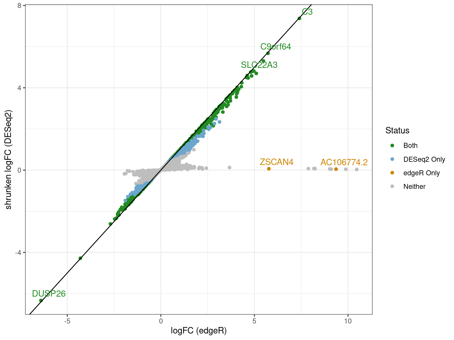
# ℹ 1,260 more rows

Comparison of Approaches

• Using the most conservative analyses
• Genes along zero for DESeq2 were a result of shrinkage

Export Results

• Save the DGEList using the following

write_rds(dge_filter, here::here("data/dge_filter.rds"))

• Save the edgeR results using the following

write_rds(res_treatM, here::here("data/res_treatM.rds"))

Conclusion

• DESeq2 data structures integrate nicely with other Bioconductor packages
• edgeR can also handle SummarizedExperiment objects (mostly)
• No right or wrong method or data classes to use
  • Results were still broadly consistent
• DESeq2 also has many options for parameter/model choice not covered here

• SummarizedExperiment objects share much with SingleCellExperiment objects
• Have helped with multiple analyses & seem preferable to Seurat (IMHO)
  • Seurat is everywhere but I spend a lot of time debugging for people

References

Liao, Yang, Gordon K Smyth, and Wei Shi. 2014. “featureCounts: An Efficient General Purpose Program for Assigning Sequence Reads to Genomic Features.” Bioinformatics 30 (7): 923–30.

Liu, Juli, Shiyong Wu, Yucheng Zhang, Cheng Wang, Sheng Liu, Jun Wan, and Lei Yang. 2023. “SARS-CoV-2 Viral Genes Nsp6, Nsp8, and M Compromise Cellular ATP Levels to Impair Survival and Function of Human Pluripotent Stem Cell-Derived Cardiomyocytes.” Stem Cell Res. Ther. 14 (1): 249.

Love, Michael I., Wolfgang Huber, and Simon Anders. 2014. “Moderated Estimation of Fold Change and Dispersion for RNA-Seq Data with DESeq2.” Genome Biology 15: 550. https://doi.org/10.1186/s13059-014-0550-8.

Lund, Steven P, Dan Nettleton, Davis J McCarthy, and Gordon K Smyth. 2012. “Detecting Differential Expression in RNA-sequence Data Using Quasi-Likelihood with Shrunken Dispersion Estimates.” Stat. Appl. Genet. Mol. Biol. 11 (5).

McCarthy, Davis J, and Gordon K Smyth. 2009. “Testing Significance Relative to a Fold-Change Threshold Is a TREAT.” Bioinformatics 25 (6): 765–71.

Robinson, Mark D, Davis J McCarthy, and Gordon K Smyth. 2010. “edgeR: A Bioconductor Package for Differential Expression Analysis of Digital Gene Expression Data.” Bioinformatics 26 (1): 139–40. https://doi.org/10.1093/bioinformatics/btp616.

Robinson, Mark D, and Alicia Oshlack. 2010. “A Scaling Normalization Method for Differential Expression Analysis of RNA-seq Data.” Genome Biol. 11 (3): R25.

Zhu, Anqi, Joseph G Ibrahim, and Michael I Love. 2019. “Heavy-Tailed Prior Distributions for Sequence Count Data: Removing the Noise and Preserving Large Differences.” Bioinformatics 35 (12): 2084–92.