Finding the Underlying Biology

RAdelaide 2024

Dr Stevie Pederson

Black Ochre Data Labs
Telethon Kids Institute

July 11, 2024

Enrichment Analysis

What is Enrichment Analysis

• Often in transcriptomics and genomics we have large lists of results
• May be genes, genomic positions etc
• How do we interpret these?
  • Should we cherry pick known high-quality candidates?
  • Should we try look for patterns within the list?

• Enrichment analysis is one strategy for looking for patterns
  • Network analysis is another approach
• Generally rely on genes can be organised into “gene sets”
  • Multiple Databases depending on your question

Multiple Approaches

• Take a ranked list of results
  \(\implies\)Are gene-sets clustered around either end

• Are genes from a specific gene-set enriched within significant results
  • Hypergeometric testing

• Can we obtain an overall value of significance for all genes within a gene-set

• No method is perfect & all have limitations
• Gene expression also appears to be highly correlated & subject to bias

Gene Ontology

• Gene Ontology (GO) Database https://www.geneontology.org/
• Restricted and highly controlled set of descriptive terms
• Terms are grouped into 3 main categories
  1. Biological Process (BP)
  2. Molecular Function (MF)
  3. Cellular Component (CC)
• Hierarchical interconnected structure within each category

Gene Ontology

Taken from https://www.geneontology.org

• Knowing how to filter results with heavily related terms can be a challenge
• Multiple pruning strategies exist

Gene Ontology

• An example using the QuickGO tool is here

KEGG

• Kyoto Encyclopedia of Genes and Genomes (KEGG)
• Exhaustive list of manually curated pathways
  1. Metabolism
  2. Genetic Information Processing
  3. Environmental Information Processing
  4. Cellular Processes
  5. Organismal Systems
  6. Human Diseases
  7. Drug Development
• Role in pathway (e.g. activation of inhibition) included

KEGG

https://www.genome.jp/pathway/hsa04010

Other Databases

• WikiPathways is an open-source analog to KEGG
  • https://www.wikipathways.org
• Reactome is highly curated, peer-reviewed database
  • https://reactome.org

• Can also use custom gene-sets
  • Results from an internal study
  • Genes matching custom genomic features

MSigDB

• The Molecular Signatures Database collects multiple databases (Liberzon et al. 2011)
  • https://www.gsea-msigdb.org/gsea/msigdb/index.jsp
  • Collected simply as gene sets without functional annotation

• H: Hallmark Gene Sets are unique to MSigDB

Gene Sets and Pathways in R

• Bioconductor provides multiple packages and tools for obtaining gene sets
  • GO.db, KEGGREST, biomaRt
• My preferred strategy is msigdbr
  • Parses MSigDb gene sets as a tibble
  • Not really built on existing Bioconductor object classes
• Best annotations are for human/mouse

msigdbr

library(tidyverse)
library(magrittr)
theme_set(theme_bw())
library(msigdbr)
msigdbr_collections()

# A tibble: 23 × 3
   gs_cat gs_subcat         num_genesets
   <chr>  <chr>                    <int>
 1 C1     ""                         299
 2 C2     "CGP"                     3384
 3 C2     "CP"                        29
 4 C2     "CP:BIOCARTA"              292
 5 C2     "CP:KEGG"                  186
 6 C2     "CP:PID"                   196
 7 C2     "CP:REACTOME"             1615
 8 C2     "CP:WIKIPATHWAYS"          664
 9 C3     "MIR:MIRDB"               2377
10 C3     "MIR:MIR_Legacy"           221
# ℹ 13 more rows

msigdbr

msigdbr_species()

# A tibble: 20 × 2
   species_name                    species_common_name                          
   <chr>                           <chr>                                        
 1 Anolis carolinensis             Carolina anole, green anole                  
 2 Bos taurus                      bovine, cattle, cow, dairy cow, domestic cat…
 3 Caenorhabditis elegans          <NA>                                         
 4 Canis lupus familiaris          dog, dogs                                    
 5 Danio rerio                     leopard danio, zebra danio, zebra fish, zebr…
 6 Drosophila melanogaster         fruit fly                                    
 7 Equus caballus                  domestic horse, equine, horse                
 8 Felis catus                     cat, cats, domestic cat                      
 9 Gallus gallus                   bantam, chicken, chickens, Gallus domesticus 
10 Homo sapiens                    human                                        
11 Macaca mulatta                  rhesus macaque, rhesus macaques, Rhesus monk…
12 Monodelphis domestica           gray short-tailed opossum                    
13 Mus musculus                    house mouse, mouse                           
14 Ornithorhynchus anatinus        duck-billed platypus, duckbill platypus, pla…
15 Pan troglodytes                 chimpanzee                                   
16 Rattus norvegicus               brown rat, Norway rat, rat, rats             
17 Saccharomyces cerevisiae        baker's yeast, brewer's yeast, S. cerevisiae 
18 Schizosaccharomyces pombe 972h- <NA>                                         
19 Sus scrofa                      pig, pigs, swine, wild boar                  
20 Xenopus tropicalis              tropical clawed frog, western clawed frog    

Setting Up An Object

• Let’s choose KEGG pathways for our analysis

kegg_tbl <- msigdbr(subcategory = "CP:KEGG")
glimpse(kegg_tbl)

Rows: 16,283
Columns: 15
$ gs_cat             <chr> "C2", "C2", "C2", "C2", "C2", "C2", "C2", "C2", "C2…
$ gs_subcat          <chr> "CP:KEGG", "CP:KEGG", "CP:KEGG", "CP:KEGG", "CP:KEG…
$ gs_name            <chr> "KEGG_ABC_TRANSPORTERS", "KEGG_ABC_TRANSPORTERS", "…
$ gene_symbol        <chr> "ABCA1", "ABCA10", "ABCA12", "ABCA13", "ABCA2", "AB…
$ entrez_gene        <int> 19, 10349, 26154, 154664, 20, 21, 24, 23461, 23460,…
$ ensembl_gene       <chr> "ENSG00000165029", "ENSG00000154263", "ENSG00000144…
$ human_gene_symbol  <chr> "ABCA1", "ABCA10", "ABCA12", "ABCA13", "ABCA2", "AB…
$ human_entrez_gene  <int> 19, 10349, 26154, 154664, 20, 21, 24, 23461, 23460,…
$ human_ensembl_gene <chr> "ENSG00000165029", "ENSG00000154263", "ENSG00000144…
$ gs_id              <chr> "M11911", "M11911", "M11911", "M11911", "M11911", "…
$ gs_pmid            <chr> "", "", "", "", "", "", "", "", "", "", "", "", "",…
$ gs_geoid           <chr> "", "", "", "", "", "", "", "", "", "", "", "", "",…
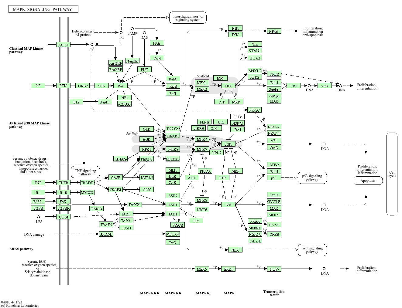
$ gs_exact_source    <chr> "hsa02010", "hsa02010", "hsa02010", "hsa02010", "hs…
$ gs_url             <chr> "http://www.genome.jp/kegg/pathway/hsa/hsa02010.htm…
$ gs_description     <chr> "ABC transporters", "ABC transporters", "ABC transp…

Setting Up An Object

• Every mapping between a gene ID and KEGG pathway is here
• Gene IDs are provided using Ensembl (EBI) and EntrezGene (NCBI)
• Gene set IDs match the specific database
• URLs are also provided
  • But can get out of date when databases reconfigure

Comparing To Our Data

res_treatM <- read_rds("data/res_treatM.rds") %>% 
  mutate(ensembl_gene = str_extract(gene_id, "ENSG[0-9]+")) # Remove version numbers
kegg_tbl %>% 
  summarise(
    gs_size = dplyr::n(),
    detected = sum(ensembl_gene %in% res_treatM$ensembl_gene),
    .by = gs_name
  ) %>% 
  mutate(prop_detected = detected / gs_size) %>% 
  arrange(prop_detected)

# A tibble: 186 × 4
   gs_name                                        gs_size detected prop_detected
   <chr>                                            <int>    <int>         <dbl>
 1 KEGG_ASTHMA                                        113        2        0.0177
 2 KEGG_GRAFT_VERSUS_HOST_DISEASE                     314        7        0.0223
 3 KEGG_OLFACTORY_TRANSDUCTION                        523       19        0.0363
 4 KEGG_AUTOIMMUNE_THYROID_DISEASE                    166        7        0.0422
 5 KEGG_ALLOGRAFT_REJECTION                           157        7        0.0446
 6 KEGG_ANTIGEN_PROCESSING_AND_PRESENTATION           535       30        0.0561
 7 KEGG_TYPE_I_DIABETES_MELLITUS                      170       12        0.0706
 8 KEGG_INTESTINAL_IMMUNE_NETWORK_FOR_IGA_PRODUC…     125        9        0.072 
 9 KEGG_TASTE_TRANSDUCTION                             89       10        0.112 
10 KEGG_NATURAL_KILLER_CELL_MEDIATED_CYTOTOXICITY     465       62        0.133 
# ℹ 176 more rows

Comparing To Our Data

• Gene sets should be chosen wisely
  • If few genes from a gene set are detected
    \(\implies\)may not be suitable for cell-type under investigation
• Should we restrict gene-sets to genes detected in our data?

• This can impact the analysis depending on the approach taken

• My take is that we should. For enrichment testing then we’re comparing changed vs unchanged in the candidate genes. Otherwise, we’re confounding detected with changed

Cleaning The Database

kegg_tbl <- kegg_tbl %>% 
  dplyr::filter(
    sum(ensembl_gene %in% res_treatM$ensembl_gene) >  0.05 * dplyr::n(),
    .by = gs_name
  ) %>% 
  dplyr::filter(
    ensembl_gene %in% res_treatM$ensembl_gene
  )

A Cautionary Limitation

• Not all genes are annotated to a gene set or pathway
• Well-studied genes are annotated to gene sets
  \(\implies\) their pathways become interesting
  \(\implies\) studied further
  \(\implies\) rinse & repeat

dplyr::filter(kegg_tbl, gene_symbol == "SNAP91") %>% nrow()

[1] 0

dplyr::filter(kegg_tbl, gene_symbol == "DUSP26") %>% nrow()

[1] 0

• This doesn’t mean these genes play an unimportant biological role!

• We can only use the available information
• Poorly studied genes can be revelations but take large sums of money

GSEA

Gene Set Enrichment Analysis

• GSEA is a formally defined algorithm (Subramanian et al. 2005)
  • Not commonly used in reference to the wider type of analysis
• Doesn’t require DEGs \(\implies\) uses a ranked list
  • Ranks based on significance only or incorporating direction

• Walks along the gene list obtaining a cumulative sum
  • Can be set to start from either end
  • Genes in a gene-set return a +ve score
  • Genes not in a gene-set return a -ve score
• Compared to permuted values to return \(p\)-values
  • Results can change on repeat runs

Gene Set Enrichment Analysis

• Can be run as a stand-alone tools
• R implementation is fgsea (Korotkevich, Sukhov, and Sergushichev 2019)
• Requires two inputs
  • A list with genes separated by gene set
  • A ranked-list of genes

library(fgsea)
kegg_by_gs <- kegg_tbl %>% 
  split(.$gs_name) %>% 
  lapply(pull, "ensembl_gene")
length(kegg_by_gs)

[1] 181

Gene Set Enrichment Analysis

• To make a directional ranked list
  • Multiply \(-\log_{10}p\) by the sign of logFC

ranks_treatM <- res_treatM %>% 
  mutate(
    rank = -sign(logFC) * log10(PValue),
    rank = setNames(rank, ensembl_gene)
  ) %>% 
  arrange(rank) %>% 
  pull(rank)
head(ranks_treatM)

ENSG00000065609 ENSG00000133878 ENSG00000118137 ENSG00000124749 ENSG00000093072 
     -12.316058      -10.005216       -7.726357       -7.383672       -7.189801 
ENSG00000167110 
      -6.815165 

Gene Set Enrichment Analysis

set.seed(101)
gsea_treatM <- fgsea(kegg_by_gs, ranks_treatM)
gsea_treatM %>% arrange(pval)

                                     pathway         pval         padj
                                      <char>        <num>        <num>
  1:                           KEGG_LYSOSOME 1.224437e-07 2.216231e-05
  2:           KEGG_ECM_RECEPTOR_INTERACTION 9.315488e-05 6.322486e-03
  3:                     KEGG_FOCAL_ADHESION 1.047926e-04 6.322486e-03
  4:    KEGG_DRUG_METABOLISM_CYTOCHROME_P450 9.649298e-04 4.366307e-02
  5: KEGG_VASCULAR_SMOOTH_MUSCLE_CONTRACTION 1.622066e-03 5.871881e-02
 ---                                                                  
177:            KEGG_CITRATE_CYCLE_TCA_CYCLE 1.000000e+00 1.000000e+00
178:                KEGG_HUNTINGTONS_DISEASE 1.000000e+00 1.000000e+00
179:                           KEGG_RIBOSOME 1.000000e+00 1.000000e+00
180:                    KEGG_RNA_DEGRADATION 1.000000e+00 1.000000e+00
181:                        KEGG_SPLICEOSOME 1.000000e+00 1.000000e+00
        log2err         ES        NES  size
          <num>      <num>      <num> <int>
  1: 0.69013246  0.7163092  1.8838119   103
  2: 0.53843410  0.7019563  1.7491321    65
  3: 0.53843410  0.5897077  1.6219153   162
  4: 0.47727082 -0.7902400 -1.7551751    21
  5: 0.45505987  0.6242822  1.5895677    77
 ---                                       
177: 0.03607300  0.2037979  0.4382494    27
178: 0.08730983 -0.2367126 -0.7463800   160
179: 0.02921031  0.1473646  0.3766860    79
180: 0.06538342 -0.1415776 -0.3838046    52
181: 0.02555230  0.1980841  0.5294166   121
                                                                                             leadingEdge
                                                                                                  <list>
  1: ENSG00000103811,ENSG00000064601,ENSG00000152056,ENSG00000107798,ENSG00000078081,ENSG00000179163,...
  2: ENSG00000186340,ENSG00000053747,ENSG00000041982,ENSG00000081052,ENSG00000132470,ENSG00000060718,...
  3: ENSG00000101335,ENSG00000186340,ENSG00000053747,ENSG00000041982,ENSG00000081052,ENSG00000166501,...
  4: ENSG00000130649,ENSG00000069535,ENSG00000134184,ENSG00000085871,ENSG00000143198,ENSG00000076258,...
  5: ENSG00000156113,ENSG00000101335,ENSG00000096433,ENSG00000166501,ENSG00000163017,ENSG00000065675,...
 ---                                                                                                    
177:                     ENSG00000138413,ENSG00000131473,ENSG00000122729,ENSG00000173599,ENSG00000166411
178: ENSG00000146592,ENSG00000198959,ENSG00000137841,ENSG00000285437,ENSG00000124172,ENSG00000228049,...
179: ENSG00000171858,ENSG00000105372,ENSG00000140988,ENSG00000185088,ENSG00000137154,ENSG00000149806,...
180: ENSG00000123737,ENSG00000272886,ENSG00000166889,ENSG00000108515,ENSG00000114127,ENSG00000138767,...
181:                                     ENSG00000132792,ENSG00000173110,ENSG00000101161,ENSG00000111786

• Using set.seed() can aid reproducibility as the same random seed is used for permutations

Gene Set Enrichment Analysis

• Adjusted p-values are FDR-adjusted by default
• Enrichment Score (ES) is the peak value from the cumulative sum
  • ES < 0 \(\implies\) result is for genes at the negative end
• Normalised Enrichment Score (NES) normalises across pathways
• The size of the gene set is also given
• The Leading Edge lists the genes more beyond the peak ES
  • Might need to convert to gene names

Gene Set Enrichment Analysis

• The enrichment score can be seen for any pathway

plotEnrichment(kegg_by_gs$KEGG_LYSOSOME, ranks_treatM) +
  ggtitle("KEGG_LYSOSOME")

Gene Set Enrichment Analysis

• Manual inspection can help us decide if we really believe the result
  • GSEA tends always find something \(\implies\) be conservative with results

library(patchwork)
gsea_treatM %>% 
  arrange(pval) %>% 
  dplyr::filter(padj < 0.05) %>% 
  dplyr::slice(1:9) %>% # Ensure we don't get more than 9
  pull(pathway) %>% 
  lapply(
    \(x) {
      lab <- str_remove_all(x, "KEGG_")
      plotEnrichment(kegg_by_gs[[x]], ranks_treatM) + ggtitle(lab)
    }
  ) %>% 
  wrap_plots()

Gene Set Enrichment Analysis

Gene Set Enrichment Analysis

• A quick summary of the results

id2symbol <- kegg_tbl %>% 
  distinct(ensembl_gene, gene_symbol) %>% 
  mutate(gene_symbol = setNames(gene_symbol, ensembl_gene)) %>% 
  pull(gene_symbol)
gsea_treatM %>% 
  arrange(pval) %>% 
  dplyr::filter(padj < 0.05) %>% 
  mutate(leSize = map_int(leadingEdge, length)) %>% 
  dplyr::select(pathway, NES, FDR = padj, size, leSize, leadingEdge) %>% 
  mutate(
    leadingEdge = lapply(leadingEdge, \(x) id2symbol[x])
  )

                                pathway       NES          FDR  size leSize
                                 <char>     <num>        <num> <int>  <int>
1:                        KEGG_LYSOSOME  1.883812 2.216231e-05   103     47
2:        KEGG_ECM_RECEPTOR_INTERACTION  1.749132 6.322486e-03    65     31
3:                  KEGG_FOCAL_ADHESION  1.621915 6.322486e-03   162     48
4: KEGG_DRUG_METABOLISM_CYTOCHROME_P450 -1.755175 4.366307e-02    21      9
                                leadingEdge
                                     <list>
1:     CTSH,CTSA,AP1S3,LIPA,LAMP3,FUCA1,...
2: THBS2,LAMA3,TNC,COL4A4,ITGB4,COL11A1,...
3:    MYL9,THBS2,LAMA3,TNC,COL4A4,PRKCB,...
4:   CYP2E1,MAOB,GSTM1,MGST2,MGST3,FMO4,...

• ECM_RECEPTOR_INTERACTION and FOCAL_ADHESION seem to be capturing a similar gene set

Gene Set Enrichment Analysis

• Show some highly ranked genes from the top-ranked pathway
  • Could choose multiple pathways & annotate genes

library(edgeR)
library(pheatmap)
dge <- read_rds("data/dge_filter.rds")
lcpm <- cpm(dge, log = TRUE)
rownames(lcpm) <- str_extract(rownames(lcpm), "ENSG[0-9]+")
le_ids <- res_treatM %>% 
  dplyr::filter(ensembl_gene %in% kegg_by_gs$KEGG_LYSOSOME, FDR < 0.1) %>% 
  pull("ensembl_gene")
lcpm[le_ids, str_subset(dge$samples$id, "(control|M)$")] %>% 
  set_rownames(id2symbol[rownames(.)]) %>% 
  apply(1, \(x) x - mean(x)) %>%
  t() %>%
  pheatmap(main = "KEGG_LYSOSOME (FDR < 0.1)")

Gene Set Enrichment Analysis

Gene Set Enrichment Analysis

• This approach has assumed that clustering by direction is biologically relevant
• Implies that up-regulated genes \(\implies\) pathway activation
• Ranks can also be prepared using significance only (\(-\log_{10}p\))
  • Effectively detects perturbed gene sets with genes at both ends

## This is pseudo-code
## Need to setup ranks_by_sig. Maybe in final DIY session?
fgsea(kegg_by_gs, ranks_by_sig, scoreType = "pos")

Final GSEA Comment

• Permutation is performed across genes
• Doesn’t take into account inter-gene correlations
  • Tends to produce spurious results

• The original GSEA took a matrix and permuted columns (i.e. sample labels)
  • Far better management of correlations
• Large number of samples is needed (n > 8)
• Is implemented as fgseaLabel()
• Similar approach for more complicated linear models in limma::romer()

Hypergeometric Approaches

Hypergeometric Testing

• Fisher’s Exact Test is a two-sided hypergeometric test
  • Test for association between groups using a \(2\times2\) table

	DEG	Not DEG
In Gene Set	\(a\)	\(b\)
Not In Gene Set	\(c\)	\(d\)

• No association \(\implies p(DEG|GS) = p(DEG|\overline{GS})\)
• One-sided tests are also plausible

Hypergeometric Testing

• Personally, I find Bioconductor testing packages cumbersome
• AnnotationDbi and GO.db contain mappings from gene to gene set
  • Often based on EnztrezGene IDs
• Many packages insist on using these (or similar strategies)
  • Feels overly complicated to me

• Could easily write our own (as for the SNP loci yesterday)
• I often use goseq (Young et al. 2010)
• Despite it’s name \(\implies\) very flexible framework
  • Albeit with a few quirks

Goseq

• goseq uses hypergeometric tests which account for bias
• Longer genes have higher counts
  • Being identified as DE can be impacted by signal level (MA plots)
• Classic hypergeometric tests are also implemented

• Analysis works with all databases
  • Requires gene sets split by gene ID
• Also requires a 0/1 named vector for DE genes

Goseq

kegg_by_gene <- kegg_tbl %>% 
  split(.$ensembl_gene) %>% 
  lapply(pull, "gs_name")
length(kegg_by_gene)

[1] 3374

de_M <- setNames(res_treatM$FDR < 0.05, res_treatM$ensembl_gene)
head(de_M)

ENSG00000065609 ENSG00000133878 ENSG00000112837 ENSG00000125730 ENSG00000112562 
           TRUE            TRUE            TRUE            TRUE            TRUE 
ENSG00000144810 
           TRUE 

Goseq

• The first step is to check the probability of a gene being DE based on gene length
  • Returns a probability weighting function (PWF) used during testing
  • Gene lengths are essential for Ensembl IDs
    \(\implies\) if not provided nullp() will try find them (very slow)

library(goseq)
pwf <- nullp(de_M, bias.data = res_treatM$length)

If not provided nullp() will try find them

Goseq

Goseq

• This object is in the required structure for enrichment testing
• The pwf column allows for biased sampling of genes

head(pwf)

                DEgenes bias.data        pwf
ENSG00000065609    TRUE      6651 0.04427687
ENSG00000133878    TRUE      1971 0.03918978
ENSG00000112837    TRUE      8654 0.04427687
ENSG00000125730    TRUE      8328 0.04427687
ENSG00000112562    TRUE      4032 0.04417537
ENSG00000144810    TRUE      9408 0.04427687

• Standard hypergeometric tests are described using red/white balls being drawn from a bag
• Biased sampling effectively allows for balls being different sizes \(\implies\) biased sampling

Goseq

• Enrichment tests are performed for over- and under-representation
• Generally we only want over-represented
• Returned p-values are not adjusted for multiple testing

goseq_M <- goseq(pwf, gene2cat = kegg_by_gene)
head(goseq_M)

                                        category over_represented_pvalue
45                 KEGG_ECM_RECEPTOR_INTERACTION            2.097988e-05
102 KEGG_NEUROACTIVE_LIGAND_RECEPTOR_INTERACTION            1.157246e-04
145                      KEGG_RETINOL_METABOLISM            2.578521e-03
14              KEGG_ARACHIDONIC_ACID_METABOLISM            3.257153e-03
54                           KEGG_FOCAL_ADHESION            3.826782e-03
40                   KEGG_DILATED_CARDIOMYOPATHY            7.525823e-03
    under_represented_pvalue numDEInCat numInCat
45                 0.9999960         13       65
102                0.9999736         13       77
145                0.9997823          4       12
14                 0.9995626          5       21
54                 0.9984649         17      162
40                 0.9977625          9       68

Goseq

• To really tidy the results

goseq_M <- goseq(pwf, gene2cat = kegg_by_gene) %>% 
  as_tibble() %>% 
  mutate(
    FDR = p.adjust(over_represented_pvalue, "fdr"),
    pDE = numDEInCat / numInCat
  ) %>% 
  dplyr::select(
    category, nDE = numDEInCat, pDE, size = numInCat, pvalue = over_represented_pvalue, FDR
  ) 
goseq_M

# A tibble: 181 × 6
   category                                      nDE   pDE  size  pvalue     FDR
   <chr>                                       <int> <dbl> <int>   <dbl>   <dbl>
 1 KEGG_ECM_RECEPTOR_INTERACTION                  13 0.2      65 2.10e-5 0.00380
 2 KEGG_NEUROACTIVE_LIGAND_RECEPTOR_INTERACTI…    13 0.169    77 1.16e-4 0.0105 
 3 KEGG_RETINOL_METABOLISM                         4 0.333    12 2.58e-3 0.139  
 4 KEGG_ARACHIDONIC_ACID_METABOLISM                5 0.238    21 3.26e-3 0.139  
 5 KEGG_FOCAL_ADHESION                            17 0.105   162 3.83e-3 0.139  
 6 KEGG_DILATED_CARDIOMYOPATHY                     9 0.132    68 7.53e-3 0.227  
 7 KEGG_CYTOKINE_CYTOKINE_RECEPTOR_INTERACTION    10 0.119    84 9.82e-3 0.254  
 8 KEGG_HYPERTROPHIC_CARDIOMYOPATHY_HCM            8 0.129    62 1.33e-2 0.302  
 9 KEGG_CELL_ADHESION_MOLECULES_CAMS               8 0.125    64 1.59e-2 0.319  
10 KEGG_TRYPTOPHAN_METABOLISM                      4 0.190    21 2.07e-2 0.374  
# ℹ 171 more rows

Goseq

• The above objects & steps are all required
• If no bias \(\implies\) PWF should be relatively flat
• To explicitly use unbiased sampling set method = "Hypergeometric"

goseq(pwf, gene2cat = kegg_by_gene, method = "Hypergeometric") %>% 
  as_tibble() %>% 
  mutate(
    FDR = p.adjust(over_represented_pvalue, "fdr"), pDE = numDEInCat / numInCat
  ) %>% 
  dplyr::select(
    category, nDE = numDEInCat, pDE, size = numInCat, pvalue = over_represented_pvalue, FDR
  ) 

# A tibble: 181 × 6
   category                                      nDE   pDE  size  pvalue     FDR
   <chr>                                       <int> <dbl> <int>   <dbl>   <dbl>
 1 KEGG_ECM_RECEPTOR_INTERACTION                  13 0.2      65 1.71e-5 0.00309
 2 KEGG_NEUROACTIVE_LIGAND_RECEPTOR_INTERACTI…    13 0.169    77 1.11e-4 0.0100 
 3 KEGG_RETINOL_METABOLISM                         4 0.333    12 2.39e-3 0.126  
 4 KEGG_FOCAL_ADHESION                            17 0.105   162 3.31e-3 0.126  
 5 KEGG_ARACHIDONIC_ACID_METABOLISM                5 0.238    21 3.48e-3 0.126  
 6 KEGG_DILATED_CARDIOMYOPATHY                     9 0.132    68 7.15e-3 0.216  
 7 KEGG_CYTOKINE_CYTOKINE_RECEPTOR_INTERACTION    10 0.119    84 9.85e-3 0.255  
 8 KEGG_HYPERTROPHIC_CARDIOMYOPATHY_HCM            8 0.129    62 1.28e-2 0.289  
 9 KEGG_CELL_ADHESION_MOLECULES_CAMS               8 0.125    64 1.54e-2 0.309  
10 KEGG_TRYPTOPHAN_METABOLISM                      4 0.190    21 2.01e-2 0.364  
# ℹ 171 more rows

Very similar for this dataset but still slightly lower p-values

Testing For Overall
DE Across A Gene Set

Camera

• One final method is to test for an overall trend towards DE across a gene set
• camera() can incorporate inter-gene correlations (Wu and Smyth 2012)
  • Default is to use a fixed value of 0.01

library(limma)
cameraPR(ranks_treatM, kegg_by_gs) %>% head()

                                          NGenes Direction       PValue
KEGG_ECM_RECEPTOR_INTERACTION                 65        Up 3.068526e-09
KEGG_HEMATOPOIETIC_CELL_LINEAGE               25        Up 2.896232e-06
KEGG_MATURITY_ONSET_DIABETES_OF_THE_YOUNG      5      Down 4.567113e-05
KEGG_DRUG_METABOLISM_CYTOCHROME_P450          21      Down 1.470574e-04
KEGG_LYSOSOME                                103        Up 2.277758e-04
KEGG_FOCAL_ADHESION                          162        Up 3.305249e-04
                                                   FDR
KEGG_ECM_RECEPTOR_INTERACTION             5.554031e-07
KEGG_HEMATOPOIETIC_CELL_LINEAGE           2.621090e-04
KEGG_MATURITY_ONSET_DIABETES_OF_THE_YOUNG 2.755492e-03
KEGG_DRUG_METABOLISM_CYTOCHROME_P450      6.654348e-03
KEGG_LYSOSOME                             8.245483e-03
KEGG_FOCAL_ADHESION                       9.970835e-03

Camera

• Correlations can be estimated more accurately from the data
• Requires the complete matrix (log-transformed), design matrix etc
  • The default (\(\rho = 0.01\)) is relatively conservative

• Are genes moving together the actual signal we want?
  • When running with accurate correlations nothing is ever significant

Closing Comments

• Chose KEGG today for simplicity (~180 pathways)
• Often choose multiple sources
• Redundancy between gene sets can be a non-trivial problem
  • No perfect solution
  • Pruning before testing or before presenting results?

Closing Comments

• All methods explored today ignored pathway topology
• KEGG and WikiPathways include topology
  • Can give insight into a pathway being inhibited or activated
  • Not just over-represented

• SPIA is the a popular strategy but concerns over handling of topologies
  • For paired samples sSNAPPY handles topology well (Liu et al. 2024)

Closing Comments

• Visualisation can also be more challenging
• What do we want to show?
  • Results clustered by similarity?
  • Results compared across data sets?
  • Proportion/Number of DE genes?
  • Expression patterns within a single gene set?

Closing Comments

• We often use an FDR of 0.05 during DGE analysis
  • Allows ~5% of noise into our data
  • Biological signal should swamp the noise

• Is an FDR-adjustment best for enrichment testing?
• Conservative approaches may be best

• Really only the beginning of the next analysis
  • Requires careful discussion with biological domain experts

References

Korotkevich, Gennady, Vladimir Sukhov, and Alexey Sergushichev. 2019. “Fast Gene Set Enrichment Analysis.” bioRxiv. https://doi.org/10.1101/060012.

Liberzon, Arthur, Aravind Subramanian, Reid Pinchback, Helga Thorvaldsdóttir, Pablo Tamayo, and Jill P Mesirov. 2011. “Molecular Signatures Database (MSigDB) 3.0.” Bioinformatics 27 (12): 1739–40.

Liu, Wenjun, Ville-Petteri Mäkinen, Wayne D Tilley, and Stephen M Pederson. 2024. “sSNAPPY: An R/Bioconductor Package for Single-Sample Directional Pathway Perturbation Analysis.” F1000Res. 13 (628): 628.

Subramanian, Aravind, Pablo Tamayo, Vamsi K Mootha, Sayan Mukherjee, Benjamin L Ebert, Michael A Gillette, Amanda Paulovich, et al. 2005. “Gene Set Enrichment Analysis: A Knowledge-Based Approach for Interpreting Genome-Wide Expression Profiles.” Proc. Natl. Acad. Sci. U. S. A. 102 (43): 15545–50.

Wu, Di, and Gordon K Smyth. 2012. “Camera: A Competitive Gene Set Test Accounting for Inter-Gene Correlation.” Nucleic Acids Res. 40 (17): e133.

Young, Matthew D, Matthew J Wakefield, Gordon K Smyth, and Alicia Oshlack. 2010. “Gene Ontology Analysis for RNA-seq: Accounting for Selection Bias.” Genome Biol. 11 (2): R14.