Exploring Data

RAdelaide 2024

Dr Stevie Pederson

Black Ochre Data Labs
Telethon Kids Institute

July 9, 2024

Exploring Our Data

Exploring Data

Now we have loaded some data into R

What does it look like?
Can we obtain summary tables?

We’ll start with some basic approaches $\rightarrow$ more sophisticated

Basic Plotting

R comes with some basic plotting capabilities
Can be easy to quickly explore $\rightarrow$ difficult to tweak
Later we’ll thoroughly explore ggplot2
- Is now the gold standard for data visualisation

plot() is useful for quick x vs. y plots
boxplot() is also fairly intuitive

Basic Plotting

The values in any column can be obtained using $

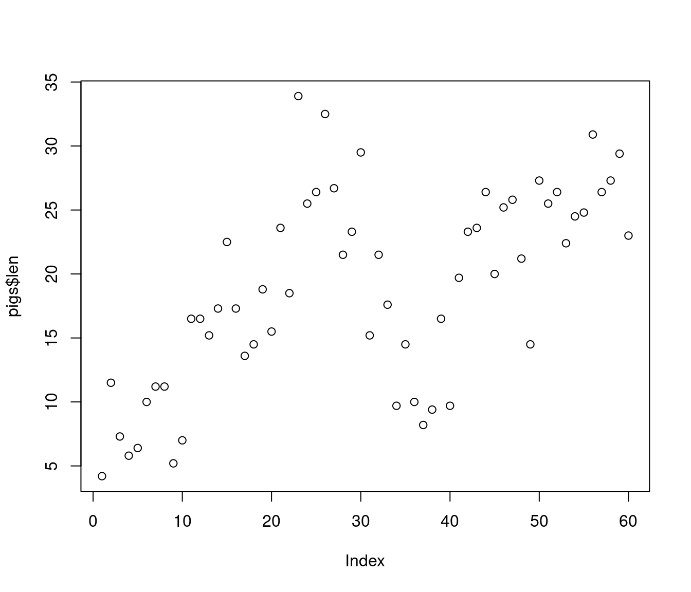
## Look at all of the odontoblast lengths
pigs$len

 [1]  4.2 11.5  7.3  5.8  6.4 10.0 11.2 11.2  5.2  7.0 16.5 16.5 15.2 17.3 22.5
[16] 17.3 13.6 14.5 18.8 15.5 23.6 18.5 33.9 25.5 26.4 32.5 26.7 21.5 23.3 29.5
[31] 15.2 21.5 17.6  9.7 14.5 10.0  8.2  9.4 16.5  9.7 19.7 23.3 23.6 26.4 20.0
[46] 25.2 25.8 21.2 14.5 27.3 25.5 26.4 22.4 24.5 24.8 30.9 26.4 27.3 29.4 23.0

We’ll discuss in great (!!!) detail tomorrow

Basic Plotting

Passing this to plot() will plot the values in order

plot(pigs$len)

Basic Boxplots

To make a boxplot we can plot len as our response variable
- Could take either supp or dose as the predictor
R uses formula syntax
- len ~ supp $\implies$ len depends on supp

## Show length as being dependent on supp
boxplot(len ~ supp, data = pigs)

Try changing supp to dose

Basic Boxplots

We can show len as depending on both using +

## Show length as being dependent on 
## both supp & dose
boxplot(len ~ supp + dose, data = pigs)

Basic Plotting

Many more options e.g. hist()

p <- c(runif(1e5), rbeta(1e4, 0.5, 1))
hist(p, breaks = 100)

ggplot2 is generally superior

Exploring Data Using `dplyr`

Introducing `dplyr`

dplyr is a core tidyverse package
- Always loaded with library(tidyverse)
Amazingly useful for
- Exploring Data
- Cleaning (i.e. tidying) Data
- Modifying & Manipulating Data
- Summarising Data
Contains many Excel-like functions

Sorting Data

By default, pigs is in the order we loaded it
Can we sort by len?

The function arrange()

Sorting Data

Here we call the function arrange()
- The data.frame is the first argument
- Any of the column names can then be passed after this

## Sort by length
arrange(pigs, len)

# A tibble: 60 × 3
     len supp  dose 
   <dbl> <chr> <chr>
 1   4.2 VC    Low  
 2   5.2 VC    Low  
 3   5.8 VC    Low  
 4   6.4 VC    Low  
 5   7   VC    Low  
 6   7.3 VC    Low  
 7   8.2 OJ    Low  
 8   9.4 OJ    Low  
 9   9.7 OJ    Low  
10   9.7 OJ    Low  
# ℹ 50 more rows

Sorting Data

Have we changed the original object?

Hint: To create an object in R we use objectName <- data

Sorting Data

Sorting is done in increasing order by default
To sort in descending order
$\implies$ wrap the column name inside the function desc()

## Sort by length, in descending order
arrange(pigs, desc(len))

# A tibble: 60 × 3
     len supp  dose 
   <dbl> <chr> <chr>
 1  33.9 VC    High 
 2  32.5 VC    High 
 3  30.9 OJ    High 
 4  29.5 VC    High 
 5  29.4 OJ    High 
 6  27.3 OJ    Med  
 7  27.3 OJ    High 
 8  26.7 VC    High 
 9  26.4 VC    High 
10  26.4 OJ    Med  
# ℹ 50 more rows

Filtering Data

dplyr also contains the function filter()

## Just subset to the high dose
filter(pigs, dose == "High")

# A tibble: 20 × 3
     len supp  dose 
   <dbl> <chr> <chr>
 1  23.6 VC    High 
 2  18.5 VC    High 
 3  33.9 VC    High 
 4  25.5 VC    High 
 5  26.4 VC    High 
 6  32.5 VC    High 
 7  26.7 VC    High 
 8  21.5 VC    High 
 9  23.3 VC    High 
10  29.5 VC    High 
11  25.5 OJ    High 
12  26.4 OJ    High 
13  22.4 OJ    High 
14  24.5 OJ    High 
15  24.8 OJ    High 
16  30.9 OJ    High 
17  26.4 OJ    High 
18  27.3 OJ    High 
19  29.4 OJ    High 
20  23   OJ    High

Filtering Data

Behind the scenes a logical test has been applied
Can only return the values TRUE or FALSE

1:5 > 2

[1] FALSE FALSE  TRUE  TRUE  TRUE

The symbol == applies the test is equal to

1:5 == 2

[1] FALSE  TRUE FALSE FALSE FALSE

The converse is != $\implies$ is NOT equal to

1:5 != 2

[1]  TRUE FALSE  TRUE  TRUE  TRUE

Filtering Data

We could exclude the high dose values instead

filter(pigs, dose != "High")

# A tibble: 40 × 3
     len supp  dose 
   <dbl> <chr> <chr>
 1   4.2 VC    Low  
 2  11.5 VC    Low  
 3   7.3 VC    Low  
 4   5.8 VC    Low  
 5   6.4 VC    Low  
 6  10   VC    Low  
 7  11.2 VC    Low  
 8  11.2 VC    Low  
 9   5.2 VC    Low  
10   7   VC    Low  
# ℹ 30 more rows

Filtering Data

Multiple filters can be separated by a comma

filter(pigs, dose == "High", supp == "OJ")

# A tibble: 10 × 3
     len supp  dose 
   <dbl> <chr> <chr>
 1  25.5 OJ    High 
 2  26.4 OJ    High 
 3  22.4 OJ    High 
 4  24.5 OJ    High 
 5  24.8 OJ    High 
 6  30.9 OJ    High 
 7  26.4 OJ    High 
 8  27.3 OJ    High 
 9  29.4 OJ    High 
10  23   OJ    High

Filtering Data

Can also filter on numeric values

filter(pigs, len > 20)

# A tibble: 28 × 3
     len supp  dose 
   <dbl> <chr> <chr>
 1  22.5 VC    Med  
 2  23.6 VC    High 
 3  33.9 VC    High 
 4  25.5 VC    High 
 5  26.4 VC    High 
 6  32.5 VC    High 
 7  26.7 VC    High 
 8  21.5 VC    High 
 9  23.3 VC    High 
10  29.5 VC    High 
# ℹ 18 more rows

Combining Functions

Can we filter then sort?
- Without modifying the original data?

We need to pass the output of one function into the next

Often referred to as piping data
- Very familiar for those who know bash (|)

Combining Functions

Two options in R

The native pipe |>
- Introduced in R v4.1 (2021)
The magrittr pipe %>%
- Introduced in the package magrittr (2014)

Both behave similarly
Code pre-2021 will always use %>%
Code post-2021 may use either

The package `magrittr`

The Treachery of Images, Rene Magritte, 1929

The package `magrittr`

I personally prefer %>% so we will use today
%>% is loaded by dplyr from the package magrittr
- The package implements some other useful functions
- Beyond the scope of today (probably)

Combining Functions

Both |> and %>% take the output of one function
$\implies$ place it as the first argument of a second
Like sticking a pipe on the output of one $\rightarrow$ connecting it to the input of another

Compare the pair

arrange(pigs, len)

# A tibble: 60 × 3
     len supp  dose 
   <dbl> <chr> <chr>
 1   4.2 VC    Low  
 2   5.2 VC    Low  
 3   5.8 VC    Low  
 4   6.4 VC    Low  
 5   7   VC    Low  
 6   7.3 VC    Low  
 7   8.2 OJ    Low  
 8   9.4 OJ    Low  
 9   9.7 OJ    Low  
10   9.7 OJ    Low  
# ℹ 50 more rows

pigs %>% arrange(len)

# A tibble: 60 × 3
     len supp  dose 
   <dbl> <chr> <chr>
 1   4.2 VC    Low  
 2   5.2 VC    Low  
 3   5.8 VC    Low  
 4   6.4 VC    Low  
 5   7   VC    Low  
 6   7.3 VC    Low  
 7   8.2 OJ    Low  
 8   9.4 OJ    Low  
 9   9.7 OJ    Low  
10   9.7 OJ    Low  
# ℹ 50 more rows

Combining Functions

Now we can join multiple functions together

pigs %>% 
  filter(supp == "OJ") %>% 
  arrange(len)

Calling pigs returns the object pigs
We filter this input filter(supp == "OJ")
Arrange the filtered object by arrange(len)

Combining Functions

Note how I wrote every function on a new line

pigs %>% 
  filter(supp == "OJ") %>% 
  arrange(len)

Makes every step clear to the reader
Can easily comment a line out in the middle
- Shortcut is Ctrl/Cmd + Shift + C
RStudio will automatically indent
- You can see where the steps start >$\implies$ where the process continues

Adding Columns Using `mutate()`

The function mutate() can be used to add columns
- Can also modify existing columns

pigs %>% 
  arrange(len) %>% 
  mutate(rank = rank(len))

# A tibble: 60 × 4
     len supp  dose   rank
   <dbl> <chr> <chr> <dbl>
 1   4.2 VC    Low     1  
 2   5.2 VC    Low     2  
 3   5.8 VC    Low     3  
 4   6.4 VC    Low     4  
 5   7   VC    Low     5  
 6   7.3 VC    Low     6  
 7   8.2 OJ    Low     7  
 8   9.4 OJ    Low     8  
 9   9.7 OJ    Low     9.5
10   9.7 OJ    Low     9.5
# ℹ 50 more rows

Adding Columns Using `mutate()`

Columns are added sequentially
Can refer to them when adding any further columns

pigs %>% 
  mutate(
    rank = rank(len),
    quantile = rank / max(rank)
  )

# A tibble: 60 × 5
     len supp  dose   rank quantile
   <dbl> <chr> <chr> <dbl>    <dbl>
 1   4.2 VC    Low     1     0.0167
 2  11.5 VC    Low    15     0.25  
 3   7.3 VC    Low     6     0.1   
 4   5.8 VC    Low     3     0.05  
 5   6.4 VC    Low     4     0.0667
 6  10   VC    Low    11.5   0.192 
 7  11.2 VC    Low    13.5   0.225 
 8  11.2 VC    Low    13.5   0.225 
 9   5.2 VC    Low     2     0.0333
10   7   VC    Low     5     0.0833
# ℹ 50 more rows

Choosing Rows

slice() can be used to choose specific rows by position
- Will never select rows beyond the range of the data
filter() selects rows by values

pigs %>% 
  slice(1:5)

# A tibble: 5 × 3
    len supp  dose 
  <dbl> <chr> <chr>
1   4.2 VC    Low  
2  11.5 VC    Low  
3   7.3 VC    Low  
4   5.8 VC    Low  
5   6.4 VC    Low

Choosing Rows

Can easily grab values for sorted data
$\implies$ the 5 with shortest odontoblasts

pigs %>% 
  arrange(len) %>% 
  slice(1:5)

# A tibble: 5 × 3
    len supp  dose 
  <dbl> <chr> <chr>
1   4.2 VC    Low  
2   5.2 VC    Low  
3   5.8 VC    Low  
4   6.4 VC    Low  
5   7   VC    Low

Choosing Columns Using `select()`

The function select() can be used to select specific columns
- One of the “heavy-lifters” of dpylr

pigs %>% 
  select(len)

# A tibble: 60 × 1
     len
   <dbl>
 1   4.2
 2  11.5
 3   7.3
 4   5.8
 5   6.4
 6  10  
 7  11.2
 8  11.2
 9   5.2
10   7  
# ℹ 50 more rows

Choosing Columns Using `select()`

Very useful for reordering columns when creating tables

pigs %>% 
  select(supp, dose, len)

# A tibble: 60 × 3
   supp  dose    len
   <chr> <chr> <dbl>
 1 VC    Low     4.2
 2 VC    Low    11.5
 3 VC    Low     7.3
 4 VC    Low     5.8
 5 VC    Low     6.4
 6 VC    Low    10  
 7 VC    Low    11.2
 8 VC    Low    11.2
 9 VC    Low     5.2
10 VC    Low     7  
# ℹ 50 more rows

Choosing Columns Using `select()`

Remove columns by placing - before the name

pigs %>% 
  mutate(
    rank = rank(len),
    quantile = rank / max(rank)
  ) %>% 
  select(-rank)

# A tibble: 60 × 4
     len supp  dose  quantile
   <dbl> <chr> <chr>    <dbl>
 1   4.2 VC    Low     0.0167
 2  11.5 VC    Low     0.25  
 3   7.3 VC    Low     0.1   
 4   5.8 VC    Low     0.05  
 5   6.4 VC    Low     0.0667
 6  10   VC    Low     0.192 
 7  11.2 VC    Low     0.225 
 8  11.2 VC    Low     0.225 
 9   5.2 VC    Low     0.0333
10   7   VC    Low     0.0833
# ℹ 50 more rows

Choosing Columns Using `select()`

Or we can just select everything but that column

pigs %>% 
  mutate(
    rank = rank(len),
    quantile = rank / max(rank)
  ) %>% 
  select(supp, dose, len, quantile)

# A tibble: 60 × 4
   supp  dose    len quantile
   <chr> <chr> <dbl>    <dbl>
 1 VC    Low     4.2   0.0167
 2 VC    Low    11.5   0.25  
 3 VC    Low     7.3   0.1   
 4 VC    Low     5.8   0.05  
 5 VC    Low     6.4   0.0667
 6 VC    Low    10     0.192 
 7 VC    Low    11.2   0.225 
 8 VC    Low    11.2   0.225 
 9 VC    Low     5.2   0.0333
10 VC    Low     7     0.0833
# ℹ 50 more rows

Using Helpers

The package tidyselect provides helpers to select by pattern
starts_with(), ends_with(), contains(), everything()

pigs %>% 
  select(starts_with("d"))

# A tibble: 60 × 1
   dose 
   <chr>
 1 Low  
 2 Low  
 3 Low  
 4 Low  
 5 Low  
 6 Low  
 7 Low  
 8 Low  
 9 Low  
10 Low  
# ℹ 50 more rows

Using Helpers

pigs %>% 
  select(ends_with("n"))

# A tibble: 60 × 1
     len
   <dbl>
 1   4.2
 2  11.5
 3   7.3
 4   5.8
 5   6.4
 6  10  
 7  11.2
 8  11.2
 9   5.2
10   7  
# ℹ 50 more rows

Using Helpers

pigs %>% 
  select(contains("e"))

# A tibble: 60 × 2
     len dose 
   <dbl> <chr>
 1   4.2 Low  
 2  11.5 Low  
 3   7.3 Low  
 4   5.8 Low  
 5   6.4 Low  
 6  10   Low  
 7  11.2 Low  
 8  11.2 Low  
 9   5.2 Low  
10   7   Low  
# ℹ 50 more rows

Using Helpers

everything() is great for putting columns first then the rest…

pigs %>% 
  mutate(
    rank = rank(len),
    quantile = rank / max(rank)
  ) %>% 
  select(supp, dose, everything())

# A tibble: 60 × 5
   supp  dose    len  rank quantile
   <chr> <chr> <dbl> <dbl>    <dbl>
 1 VC    Low     4.2   1     0.0167
 2 VC    Low    11.5  15     0.25  
 3 VC    Low     7.3   6     0.1   
 4 VC    Low     5.8   3     0.05  
 5 VC    Low     6.4   4     0.0667
 6 VC    Low    10    11.5   0.192 
 7 VC    Low    11.2  13.5   0.225 
 8 VC    Low    11.2  13.5   0.225 
 9 VC    Low     5.2   2     0.0333
10 VC    Low     7     5     0.0833
# ℹ 50 more rows

Removing Repeated Entries

distinct() will reduce the data to unique values
- One or more columns
Will drop any other columns by default

pigs %>% 
  distinct(supp, dose)

# A tibble: 6 × 2
  supp  dose 
  <chr> <chr>
1 VC    Low  
2 VC    Med  
3 VC    High 
4 OJ    Low  
5 OJ    Med  
6 OJ    High

Removing Repeated Entries

Adding .keep_all will keep the first value in all other columns
If we sort by len first >$\implies$ returns the lowest value for each combination

pigs %>% 
  arrange(len) %>% 
  distinct(supp, dose, .keep_all = TRUE)

# A tibble: 6 × 3
    len supp  dose 
  <dbl> <chr> <chr>
1   4.2 VC    Low  
2   8.2 OJ    Low  
3  13.6 VC    Med  
4  14.5 OJ    Med  
5  18.5 VC    High 
6  22.4 OJ    High

Creating Summaries

Summaries ‘on-the-fly’ without creating new objects
Filtering for OJ allows us to get some key summary statistics

pigs %>% 
  filter(supp == "OJ") %>% 
  summarise(
    mn = mean(len),
    sd = sd(len)
  )

# A tibble: 1 × 2
     mn    sd
  <dbl> <dbl>
1  20.7  6.61

Creating Summaries

Summaries can be grouped by using the .by argument

pigs %>% 
  summarise(
    mn = mean(len),
    sd = sd(len),
    .by = supp
  )

# A tibble: 2 × 3
  supp     mn    sd
  <chr> <dbl> <dbl>
1 VC     17.0  8.27
2 OJ     20.7  6.61

Creating Summaries

Summaries can be grouped by multiple columns

pigs %>% 
  summarise(
    mn = mean(len),
    sd = sd(len),
    .by = c(supp, dose)
  )

# A tibble: 6 × 4
  supp  dose     mn    sd
  <chr> <chr> <dbl> <dbl>
1 VC    Low    7.98  2.75
2 VC    Med   16.8   2.52
3 VC    High  26.1   4.80
4 OJ    Low   13.2   4.46
5 OJ    Med   22.7   3.91
6 OJ    High  26.1   2.66

Note the use of c(supp, dose)

Joining Values Using `c()`

In R the function c() stands for combine
- Or maybe concatenate…?
- Both terms are used on the help page
Joins multiple values into a single vector
- We’ll examine vectors thoroughly tomorrow

c(1, 20)

[1]  1 20

Summary of Main Functions

filter(), arrange() for excel-like sorting & filtering
slice() for rows and select() for columns
- helpers include: ends_with(), starts_with(), contains(), everything()
mutate() to modify or add columns
distinct() for removing repeat entries
summarise() to obtain summary tables

Combining Multiple Data Frames

Combining Data Frames

We often need to combine data from multiple sources
bind_rows() can combine the rows from multiple data frames
- Like stacking them on top of each other
- Must have similar structure to be relevant
- Use case may be separate measurement sets held in different csv files

left_join() can join two data frames
- Looks for shared columns & common values
- Appends extra columns onto an existing object

Combining Data Frames

Grabbing the first and last 5 rows as an example
(Probably not very useful for pigs…)

bind_rows(
  slice(pigs, 1:5),
  slice(pigs, 55:60)
)

# A tibble: 11 × 3
     len supp  dose 
   <dbl> <chr> <chr>
 1   4.2 VC    Low  
 2  11.5 VC    Low  
 3   7.3 VC    Low  
 4   5.8 VC    Low  
 5   6.4 VC    Low  
 6  24.8 OJ    High 
 7  30.9 OJ    High 
 8  26.4 OJ    High 
 9  27.3 OJ    High 
10  29.4 OJ    High 
11  23   OJ    High

Combining Data Frames

If we name the data frames $\implies$ can be added as a column

bind_rows(
  top5 = slice(pigs, 1:5),
  bottom5 = slice(pigs, 55:60),
  .id = "source"
)

# A tibble: 11 × 4
   source    len supp  dose 
   <chr>   <dbl> <chr> <chr>
 1 top5      4.2 VC    Low  
 2 top5     11.5 VC    Low  
 3 top5      7.3 VC    Low  
 4 top5      5.8 VC    Low  
 5 top5      6.4 VC    Low  
 6 bottom5  24.8 OJ    High 
 7 bottom5  30.9 OJ    High 
 8 bottom5  26.4 OJ    High 
 9 bottom5  27.3 OJ    High 
10 bottom5  29.4 OJ    High 
11 bottom5  23   OJ    High

Joining Data Frames

Joining (or merging) uses shared columns between data frames
- Finds common values in the shared columns
- Best for names, labels etc (not numbers)
Appends data from one data.frame onto the other

If adding data relevant for specific rows we use *_join()
- left_join(), right_join()
- inner_join(), full_join()
If adding independent columns $\implies$ bind_cols()
- Will be no connection between data frames

Joining Data Frames

pigs isn’t great for this
We’ll use two data frames already in R

band_members

# A tibble: 3 × 2
  name  band   
  <chr> <chr>  
1 Mick  Stones 
2 John  Beatles
3 Paul  Beatles

band_instruments

# A tibble: 3 × 2
  name  plays 
  <chr> <chr> 
1 John  guitar
2 Paul  bass  
3 Keith guitar

These are similar and related
Some shared values but some differences

Joining Data

left_join() takes the first (i.e. left) data.frame as the scaffold
- Adds the second (i.e. right) data.frame
- If no matching values in the right data.frame $\implies$ NA

band_members %>% 
  left_join(band_instruments)

# A tibble: 3 × 3
  name  band    plays 
  <chr> <chr>   <chr> 
1 Mick  Stones  <NA>  
2 John  Beatles guitar
3 Paul  Beatles bass

Joining Data

right_join() takes the second (i.e. right) as the scaffold
- Adds the first (i.e. left) data.frame
- If no matching values in the left data.frame $\implies$ NA

band_members %>% 
  right_join(band_instruments)

# A tibble: 3 × 3
  name  band    plays 
  <chr> <chr>   <chr> 
1 John  Beatles guitar
2 Paul  Beatles bass  
3 Keith <NA>    guitar

Joining Data

full_join() incorporates all data combinations

band_members %>% 
  full_join(band_instruments)

# A tibble: 4 × 3
  name  band    plays 
  <chr> <chr>   <chr> 
1 Mick  Stones  <NA>  
2 John  Beatles guitar
3 Paul  Beatles bass  
4 Keith <NA>    guitar

Joining Data

inner_join() only return complete combinations

band_members %>% 
  inner_join(band_instruments)

# A tibble: 2 × 3
  name  band    plays 
  <chr> <chr>   <chr> 
1 John  Beatles guitar
2 Paul  Beatles bass

Missing Data

One final trick is case_when()
- Like a multi-level if else statement
Where the logical test is TRUE, the value on the RHS of “~” is used
- Test are conducted sequentially
- Once TRUE $\implies$ no more tests

band_members %>% 
  left_join(band_instruments) %>% 
  mutate(
    plays = case_when(
      is.na(plays) ~ "the role of a man 40 years younger",
      !is.na(plays) ~ plays
    )
  )

# A tibble: 3 × 3
  name  band    plays                             
  <chr> <chr>   <chr>                             
1 Mick  Stones  the role of a man 40 years younger
2 John  Beatles guitar                            
3 Paul  Beatles bass

Closing Comments

Many functions here have common names:
- select(), filter() etc
- Based on long-established SQL processes

Other package developers have also used these names
Can create conflicts $\implies$ code ‘inexplicably’ stops working

Closing Comments

Call directly from the package using the namespace
- dplyr::filter() instead of filter()
- dplyr::select() instead of select()
- dplyr::slice() instead of slice()
I use these three every time to be safe

A namespace is simply the list of functions made visible in a package
Calling directly from a namespace is quite acceptable
- Can look clunky but is efficient & good practice
- Very common inside package functions

Exploring Data

Exploring Our Data

Exploring Data

Basic Plotting

Basic Plotting

Basic Plotting

Basic Boxplots

Basic Boxplots

Basic Plotting

Exploring Data Using dplyr

Introducing dplyr

Sorting Data

Sorting Data

Sorting Data

Sorting Data

Filtering Data

Filtering Data

Filtering Data

Filtering Data

Filtering Data

Combining Functions

Combining Functions

Combining Functions

The package magrittr

The package magrittr

Combining Functions

Combining Functions

Combining Functions

Adding Columns Using mutate()

Adding Columns Using mutate()

Choosing Rows

Choosing Rows

Choosing Columns Using select()

Choosing Columns Using select()

Choosing Columns Using select()

Choosing Columns Using select()

Using Helpers

Using Helpers

Using Helpers

Using Helpers

Removing Repeated Entries

Removing Repeated Entries

Creating Summaries

Creating Summaries

Creating Summaries

Joining Values Using c()

Summary of Main Functions

Combining Multiple Data Frames

Combining Data Frames

Combining Data Frames

Combining Data Frames

Joining Data Frames

Joining Data Frames

Joining Data

Joining Data

Joining Data

Joining Data

Missing Data

Closing Comments

Closing Comments

Exploring Data Using `dplyr`

Introducing `dplyr`

The package `magrittr`

The package `magrittr`

Adding Columns Using `mutate()`

Adding Columns Using `mutate()`

Choosing Columns Using `select()`

Choosing Columns Using `select()`

Choosing Columns Using `select()`

Choosing Columns Using `select()`

Joining Values Using `c()`