Introductory Visualisation

RAdelaide 2024

Dr Stevie Pederson

Black Ochre Data Labs
Telethon Kids Institute

July 9, 2024

Visualisation With
`ggplot2`

The Grammar of Graphics

ggplot2 has become the industry standard for visualisation (Wickham 2016)
Core & essential part of the tidyverse
Developed by Hadley Wickham as his PhD thesis
An implementation of The Grammar of Graphics (Wilkinson 2005)
- Breaks visualisation into layers

The Grammar of Graphics

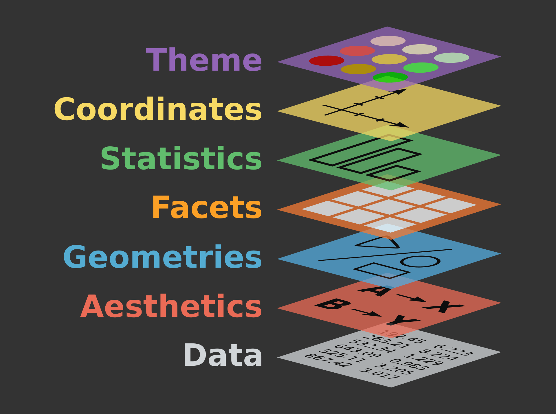
Taken from https://r.qcbs.ca/workshop03/book-en/grammar-of-graphics-gg-basics.html

The Grammar of Graphics

Everything is added in layers

Data
- Usually a data.frame (or tibble)
- Can be piped in \(\implies\) modify on the fly

Aesthetics
- x & y co-ordinates
- colour, fill, shape, size, linetype
- grouping & transparency (alpha)

Geometric Objects
- points, lines, boxplot, histogram, bars etc

Facets: Panels within plots

Statistics: Computed summaries

Coordinates
- polar, map, cartesian etc
- defaults to cartesian

Themes: overall layout
- default themes automatically applied

An Initial Example

Using the example dataset cars
Two columns:
- speed (mph)
- distance each car takes to stop
We can make a classic x vs y plot using points

The predictor (x) would be speed
The response (y) would be distance

An Initial Example

We may as well start by piping our data in

cars %>% 
  ggplot(aes(x = speed, y = dist))

We have defined the plotting aesthetics
- x & y
- Don’t need to name if passing in order
Axis limits match the data

No geometry has been specified \(\implies\) nothing was drawn

An Initial Example

To add points, we add geom_point() after calling ggplot()
- Adding + after ggplot() says “But wait! There’s more…”

cars %>%
  ggplot(aes(x = speed, y = dist)) + 
  geom_point()

An Initial Example

To add points, we add geom_point() after calling ggplot()
- Adding + after ggplot() says “But wait! There’s more…”

cars %>% # Layer 1: Data
  ggplot(aes(x = speed, y = dist)) + # Layer 2: Aesthetics
  geom_point() # Layer 3: Geometry

By default:
- Layer 4: No facets
- Layer 5: No summary statistics
- Layer 6: Cartesian co-ordinate system
- Layer 7: Crappy theme with grey background 🤮

Visualising Our Guinea Pig Data

What visualisations could we produce to inspect pigs?

Creating Our Boxplot

A starting point might be to choose dose as the predictor
len will always be the response variable

pigs %>% 
  ggplot(aes(dose, len)) +
  geom_boxplot()

Creating Our Boxplot

To incorporate the supp methods \(\implies\) add a fill aesthetic
- colour is generally applied to shape outlines

pigs %>% 
  ggplot(aes(dose, len, fill = supp)) +
  geom_boxplot()

ggplot2 will always separate multiple values/category

Creating Our Boxplot

We could also separate by supp using facet_wrap()
- Can also set the number of rows/columns

pigs %>% 
  ggplot(aes(dose, len, fill = supp)) +
  geom_boxplot() +
  facet_wrap(~supp)

Only one value/category so no shifting

Layering Geometries

We’re not restricted to one geometry
The following will add points after drawing the boxplots

pigs %>% 
  ggplot(aes(dose, len, fill = supp)) +
  geom_boxplot() +
  geom_point() +
  facet_wrap(~supp)

Layering Geometries

geom_jitter() will add a small amount of noise to separate points

pigs %>% 
  ggplot(aes(dose, len, fill = supp)) +
  geom_boxplot() +
  geom_jitter(width = 0.1, height = 0) +
  facet_wrap(~supp)

Modifying Data Prior to Plotting

dose is a clearly a categorical variable with an order
In R these are known as factors
- Categories referred to as levels
- Will learn in detail in the next session

ggplot() will automatically place character columns in alphanumeric order
Manually set the order by explicitly setting as a factor with levels

Modifying Data Prior to Plotting

Notice the column is now described as fct

pigs %>% 
  mutate(dose = factor(dose, levels = c("Low", "Med", "High")))

# A tibble: 60 × 3
     len supp  dose 
   <dbl> <chr> <fct>
 1   4.2 VC    Low  
 2  11.5 VC    Low  
 3   7.3 VC    Low  
 4   5.8 VC    Low  
 5   6.4 VC    Low  
 6  10   VC    Low  
 7  11.2 VC    Low  
 8  11.2 VC    Low  
 9   5.2 VC    Low  
10   7   VC    Low  
# ℹ 50 more rows

Modifying Data Prior to Plotting

Now boxplots will appear in order

pigs %>% 
  mutate(dose = factor(dose, levels = c("Low", "Med", "High"))) %>% 
  ggplot(aes(dose, len, fill = supp)) +
  geom_boxplot()

Modifying Data Prior to Plotting

We can also plot quantiles with a few prior steps
First rank the len values \(\implies\) turn into quantiles

pigs %>% 
  mutate(
    rank = rank(len),
    q = rank / max(rank)
  )

# A tibble: 60 × 5
     len supp  dose   rank      q
   <dbl> <chr> <chr> <dbl>  <dbl>
 1   4.2 VC    Low     1   0.0167
 2  11.5 VC    Low    15   0.25  
 3   7.3 VC    Low     6   0.1   
 4   5.8 VC    Low     3   0.05  
 5   6.4 VC    Low     4   0.0667
 6  10   VC    Low    11.5 0.192 
 7  11.2 VC    Low    13.5 0.225 
 8  11.2 VC    Low    13.5 0.225 
 9   5.2 VC    Low     2   0.0333
10   7   VC    Low     5   0.0833
# ℹ 50 more rows

Modifying Data Prior to Plotting

pigs %>% 
  mutate(
    rank = rank(len),
    q = rank / max(rank)
  ) %>% 
  ggplot(aes(len, q)) +
  geom_point()

Modifying Data Prior to Plotting

Now we could colour points by supp

pigs %>% 
  mutate(
    rank = rank(len),
    q = rank / max(rank)
  ) %>% 
  ggplot(aes(len, q, colour = supp)) +
  geom_point()

Different Layers

Modifying Data Prior to Plotting

geom_smooth() will add a line of best fit
- Aliases stat_smooth()
Automatically chosen but can be lm, loess or gam

pigs %>% 
  mutate(
    rank = rank(len),
    q = rank / max(rank)
  ) %>% 
  ggplot(aes(len, q, colour = supp)) +
  geom_point() +
  geom_smooth()

Modifying Geoms

Any aesthetic set in the call to ggplot() is passed to every subsequent layer
We can set aesthetics in a layer-specific manner
Shifting colour = supp to geom_point() will only colour points
The line of best fit will now be a single line

Modifying Geoms

pigs %>% 
  mutate(
    rank = rank(len),
    q = rank / max(rank)
  ) %>% 
  ggplot(aes(len, q)) +
  geom_point(aes(colour = supp)) +
  geom_smooth()

Modifying Geoms

Aesthetics can also be set outside of a call to aes()

pigs %>% 
  mutate(
    rank = rank(len),
    q = rank / max(rank)
  ) %>% 
  ggplot(aes(len, q)) +
  geom_point(aes(colour = supp)) +
  geom_smooth(colour = "black")

Modifying Geoms

Geoms are just regular functions with multiple arguments
The below turns off the se bands and switches to lm

pigs %>% 
  mutate(
    rank = rank(len),
    q = rank / max(rank)
  ) %>% 
  ggplot(aes(len, q)) +
  geom_point(aes(colour = supp)) +
  geom_smooth(colour = "black", se = FALSE, method = "lm")

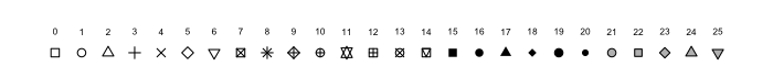
Choosing Point Shapes

Shapes have numeric codes in R
Examples are on the ?pch page
The default is 19
Can also be set as an aesthetic
size can also work either way

Choosing Point Shapes

pigs %>% 
  mutate(
    rank = rank(len),
    q = rank / max(rank)
  ) %>% 
  ggplot(aes(len, q)) +
  geom_point(aes(colour = supp), shape = 1, size = 3) +
  geom_smooth(colour = "black", se = FALSE, method = "lm")

Setting Scales

Default scales are set for x & y axes
- scale_x_continuous() & scale_y_continuous()
- Only needed when tweaking axis names, limits, labels, breaks etc
Also set scales for colours, shapes, fill etc

pigs %>% 
  mutate(
    rank = rank(len),
    q = rank / max(rank)
  ) %>% 
  ggplot(aes(len, q)) +
  geom_point(aes(colour = supp)) +
  scale_x_continuous(name = "Odontoblast Length") +
  scale_y_continuous(name = "Quantile")

Setting Scales

scale_colour_brewer() allows pre-defined palettes
- From the package RColorBrewer

pigs %>% 
  mutate(
    rank = rank(len),
    q = rank / max(rank)
  ) %>% 
  ggplot(aes(len, q)) +
  geom_point(aes(colour = supp)) +
  scale_x_continuous(name = "Odontoblast Length") +
  scale_y_continuous(name = "Quantile") +
  scale_colour_brewer(palette = "Set2", direction = -1)

RColorBrewer Palettes

Setting Scales

scale_colour_viridis_b/c/d()
- colour-blind friendly palettes
- comes in binned (_b()), continuous (_c()) or discrete (_d())
- excellent for heatmaps or showing differences across large range

pigs %>% 
  mutate(
    rank = rank(len),
    q = rank / max(rank)
  ) %>% 
  ggplot(aes(len, q)) +
  geom_point(aes(colour = supp)) +
  scale_x_continuous(name = "Odontoblast Length") +
  scale_y_continuous(name = "Quantile") +
  scale_colour_viridis_d()

Setting Scales

scale_colour_manual() takes a vector of colours
- Vectors are formed using c()
- RStudio helpfully shows you the colour!!!

pigs %>% 
  mutate(
    rank = rank(len),
    q = rank / max(rank)
  ) %>% 
  ggplot(aes(len, q)) +
  geom_point(aes(colour = supp)) +
  scale_x_continuous(name = "Odontoblast Length") +
  scale_y_continuous(name = "Quantile") +
  scale_colour_manual(values = c("orange", "navyblue"))

Themes

We can modify the overall appearance of the plot using theme()
Set panel colours, fonts, legend position etc
Hide any features we don’t want

Themes

To help us focus on the theme()
\(\implies\) save the plot as the object p

p <- pigs %>% 
  mutate(
    rank = rank(len),
    q = rank / max(rank)
  ) %>% 
  ggplot(aes(len, q)) +
  geom_point(aes(colour = supp)) +
  scale_x_continuous(name = "Odontoblast Length") +
  scale_y_continuous(name = "Quantile") +
  scale_colour_manual(values = c("orange", "navyblue"))

We can regenerate the plot by typing it’s name

Themes

ggplot2 supplies several complete themes
Applies theme_grey() by default
Try add theme_bw() after p
- This is my default

p + theme_bw()

Try a few others
- theme_void(), theme_classic(), theme_minimal()
Some are for specific use cases

Themes

We can also modify manually
Theme elements are modified using element_*() functions
- Text elements use element_text()
- Line elements use element_line()
- Box (or rectangle) elements use element_rect()
- Can disable an element entirely using element_blank()

p + theme(panel.background = element_blank())

Themes

The panel background is set using element_rect()
- colour sets the rectangle outline colour
- fill sets the rectangle fill

p + theme(panel.background = element_rect(fill = "white", colour = "grey30"))

Themes

We can set global text parameters using text = element_text()
- family, colour, size, face etc

p + 
  theme(
    panel.background = element_rect(fill = "white", colour = "grey30"),
    text = element_text(family = "serif", size = 14)
  )

Themes

Individual text-based parameters can be set similarly
Will over-ride any global setting

p + 
  theme(
    panel.background = element_rect(fill = "white", colour = "grey30"),
    text = element_text(family = "serif", size = 14),
    axis.title = element_text(face = "bold")
  )

Themes

Can also set a theme then modify further

p +
  theme_bw() +
  theme(panel.grid = element_blank())

Enormous range of setting can be controlled here

Themes

Spend a few minutes playing with the following
Try commenting out lines or changing values
Aesthetic names can be set manually using labs()
- Won’t over-write anything set in scale_x/y_continuous()

p +
  ggtitle("Odontoblast Length in Guinea Pigs") +
  labs(colour = NULL) +
  theme(
    rect = element_rect(fill = "#204080"),
    text = element_text(colour = "grey80", family = "Palatino", size = 14),
    panel.background = element_rect(fill = "steelblue4", colour = "grey80"),
    panel.grid = element_line(colour = "grey80", linetype = 2, linewidth = 1/4),
    axis.text = element_text(colour = "grey80"),
    legend.background = element_rect(fill = "steelblue4", colour = "grey80"),
    legend.key = element_rect(colour = NA),
    legend.position = "inside", 
    legend.position.inside = c(1, 0), 
    legend.justification = c(1, 0),
    plot.title = element_text(hjust = 0.5, face = "bold"),
  )

Themes

Saving Images

The simple way is click Export in the Plots pane

The way to save using code is

ggsave("myplot.png", width = 7, height = 7, units = "in")

This will always save the most recent plot by default
Output format is determined by the suffix
Try saving as a pdf…

Saving Images

I think saving using code is preferable
Modify an analysis or data \(\implies\) saved figures will also update
- This saves time & ensures reproducibility

Conclusion

A fabulous resource: https://r-graphics.org/

References

Wickham, Hadley. 2016. Ggplot2: Elegant Graphics for Data Analysis. Springer-Verlag New York. https://ggplot2.tidyverse.org.

Wilkinson, Leland. 2005. The Grammar of Graphics. Springer New York, NY. https://doi.org/https://doi.org/10.1007/0-387-28695-0.

Introductory Visualisation

Visualisation Withggplot2

The Grammar of Graphics

The Grammar of Graphics

The Grammar of Graphics

An Initial Example

An Initial Example

An Initial Example

An Initial Example

Visualising Our Guinea Pig Data

Creating Our Boxplot

Creating Our Boxplot

Creating Our Boxplot

Layering Geometries

Layering Geometries

Modifying Data Prior to Plotting

Modifying Data Prior to Plotting

Modifying Data Prior to Plotting

Modifying Data Prior to Plotting

Modifying Data Prior to Plotting

Modifying Data Prior to Plotting

Different Layers

Modifying Data Prior to Plotting

Modifying Geoms

Modifying Geoms

Modifying Geoms

Modifying Geoms

Choosing Point Shapes

Choosing Point Shapes

Setting Scales

Setting Scales

RColorBrewer Palettes

Setting Scales

Setting Scales

Themes

Themes

Themes

Themes

Themes

Themes

Themes

Themes

Themes

Themes

Themes

Saving Images

Saving Images

Conclusion

References

Visualisation With
`ggplot2`