R Markdown

RAdelaide 2024

Dr Stevie Pederson

Black Ochre Data Labs
Telethon Kids Institute

July 10, 2024

R Markdown

Writing Reports Using `rmarkdown`

rmarkdown is a cohesive way to
- Load & wrangle data
- Analyse data, including figures & tables
- Publish everything in a complete report/analysis
The package knitr is the engine behind this
- Replaced the Sweave package about 8-10 years ago

Extends the markdown language to incorporate R code

Writing Reports Using `rmarkdown`

Everything is one document
- Our analysis code embedded alongside our explanatory text
The entire analysis is performed in a fresh R Environment
- Avoids issues with saving/re-saving Workspaces
Effectively enforces code that runs sequentially

Starting With Markdown

A Brief Primer on Markdown

Markdown is a simple and elegant way to create formatted HTML
- Text is entered as plain text
- Formatting usually doesn’t appear on screen (but can)
- The parsing to HTML often occurs using pandoc
Often used for Project README files etc.
Not R-specific but is heavily-used across data-science

Go to the File drop-down menu in RStudio
New File -> Markdown File
Save As README.md

Editing Markdown

Section Headers are denoted by on or more # symbols
- # is the highest level, ## is next highest etc.

Italic text is set by enclosing text between a single asterisk (*) or underscore (_)

Bold text is set by using two asterisks (**) or two underscores (__)

Editing Markdown

Dot-point Lists are started by prefixing each line with -
- Next level indents are formed by adding 2 or 4 spaces before the next -

Numeric Lists are formed by starting a line with 1.
- Subsequent lines don’t need to be numbered in order

Editing Markdown

Let’s quickly edit our file so there’s something informative

Enter this on the top line

# RAdelaide 2024

Two lines down add this

## Day 1

Leave another blank line then add

1. Introduction to R and R Studio
2. Importing Data
3. Data Exploration
4. Data Visualisation

Editing Markdown

Underneath the list enter:

**All material** can be found at [the couse homepage](http://blackochrelabs.au/RAdelaide24/)

Here we’ve set the first two words to appear in bold font
The section in the square brackets will appear as text with a hyperlink to the site in the round brackets

Click the Preview Button and an HTML document appears
Note that README.html has also been produced
- Sites like github/gitlab render this automatically
- Obsidian also renders interactively

R Markdown

Writing Reports Using `rmarkdown`

We can output our analysis directly as:

HTML
MS Word Documents
PDF Documents (If you have $\LaTeX$ installed)
Slidy, ioslides or PowerPoint presentations

We never need to use MS Word, Excel or PowerPoint again!

Writing Reports Using `rmarkdown`

The file suffix is .Rmd
Include both markdown + embedded R code.
Create all of our figures & tables directly from the data
Data, experimental and analytic descriptions
Mathematical/Statistical equations
Nicely Formatted Results
Any other information: citations, hyperlinks etc.

Creating an R Markdown document

Let’s create our first rmarkdown document

Go to the File drop-down menu in RStudio
New File -> R Markdown…

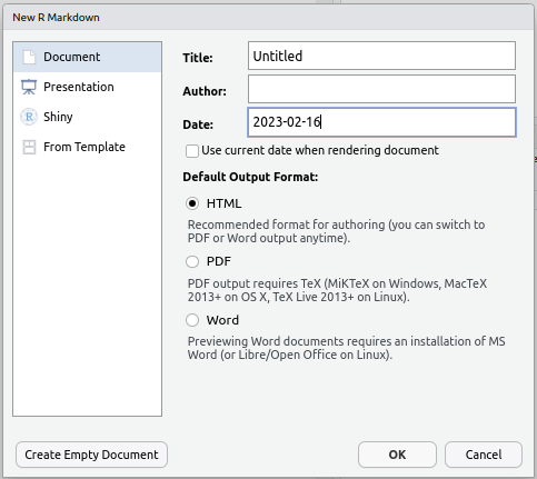
Creating an R Markdown document

Change the Title to: My First Report
Change the Author to your preferred name
Leave everything else as it is & hit OK
Save the file as RMarkdownTutorial.Rmd

Looking At The File

A header section is enclosed between the --- lines at the top

Nothing can be placed before this!
Uses YAML (YAML Ain’t Markup Language)
Editing is beyond the scope of this course
Can set custom .css files, load LaTeX packages, set parameters etc.

Looking At The File

Lines 8 to 10 are a code chunk

Chunks always begin with ```{r}
Chunks always end with ```
Executed R code goes between these two delineation marks

Chunk names are optional and directly follow the letter r
- Chunks can also be other languages (bash, python etc.)
- Here the r tells RMarkdown the chunk is an R chunk

Other parameters are set in the chunk header (e.g. do we show/hide the code)
- The master reference is here

Looking At The File

Line 12 is a Subsection Heading, starting with ##

Click the Outline symbol in the top-right of the Script Window
Chunk names are shown in italics (if set to be shown)
- Tools > Global Options > R Markdown
- Show in document outline: Sections and All Chunks
Section Names in plain text
Chunks are indented within Sections
By default Sections start with ##
- Only the Document Title should be Level 1 #

Getting Help

Check the help for a guide to the syntax.

Help > Markdown Quick Reference

Increasing numbers of # gives Section $\rightarrow$ Subsection $\rightarrow$ Subsubsection etc.
Bold is set by **Knit** (or __Knit__)
Italics can be set using a single asterisk/underline: *Italics* or _Italics_
Typewriter font is set using a single back-tick `Typewriter`

Compiling The Report

The default format is an html_document & we can change this later. Generate the default document by clicking Knit

Compiling The Report

The Viewer Pane will appear with the compiled report (probably)

Note the hyperlink to the RMarkdown website & the bold typeface for the word Knit
The R code and the results are printed for summary(cars)
The plot of temperature Vs. pressure has been embedded
The code for the plot was hidden using echo = FALSE

Compiling The Report

We could also export this as an MS Word document by clicking the small ‘down’ arrow next to the word Knit.
By default, this will be Read-Only, but can be helpful for sharing with collaborators.
Saving as a .PDF requires $\LaTeX$
- Beyond the scope of today

Making Our Own Report

Now we can modify the code to create our own analysis.

Delete everything in your R Markdown file EXCEPT the header
We’ll analyse the pigs dataset
Edit the title to be something suitable

Making Our Own Reports

What do we need for our report?

Load and describe the data using clear text explanations
- Maybe include the questions being asked by the study
Create figures which show any patterns, trends or issues
Perform an analysis
State conclusions
Send to collaborators

Making Our Own Reports

First we’ll need to load the data
- Then we can describe the data
RMarkdown always compiles from the directory it is in
- File paths should be relative to this

My “first” real chunk always loads the packages we need

Creating a Code Chunk

Alt+Ctrl+I creates a new chunk on Windows/Linux
- Cmd+Option+I on OSX

Type load-packages next to the ```{r
- This is the chunk name
- Really helpful habit to form

Enter library(tidyverse) in the chunk body
- We’ll add other packages as we go

Knit…

Dealing With Messages

The tidyverse is a little too helpful sometimes
- These messages look horrible in a final report
- Are telling us which packages/version tidyverse has loaded
- Also informing us of conflicts (e.g. dplyr::filter Vs. stats::filter)
- Can be helpful when running an interactive session
We can hide these from our report

Dealing With Messages

Go to the top of your file (below the YAML)
Create a new chunk
Name it setup
Place a comma after setup and add include = FALSE
- This will hide the chunk from the report

In the chunk body add knitr::opts_chunk$set(message = FALSE)
- This sets a global parameter for all chunks
- i.e. Don’t print “helpful” messages

Knit…

Making Our Own Reports

I like to load all data straight after loading packages
Gets the entire workflow sorted at the beginning
Alerts to any problems early

Below the load-packages chunk:

Create a new chunk
Name it load-data
In the chunk body load pigs using read_csv()

pigs <- read_csv("data/pigs.csv") %>% 
    mutate(
        dose = factor(dose, levels = c("Low", "Med", "High")),
        supp = factor(supp, levels = c("VC", "OJ"))
    )

Describing Data

Now let’s add a section header for our analysis to start the report

Type ## Data Description after the header and after leaving a blank line
Use your own words to describe the data
- Consider things like how many participants, different methods, measures we have etc.

60 guinea pigs were given vitamin C, either in their drinking water in via orange juice. 3 dose levels were given representing low, medium and high doses. Odontoblast length was measured in order to assess the impacts on tooth growth

Describing Data

In my version, I mentioned the study size
We can take this directly from the data
- Very useful as participants change
nrow(pigs) would give us the number of pigs

Replace the number 60 in your description with `r nrow(pigs)`

Knit…

Visualising The Data

The next step might be to visualise the data using a boxplot
Start a new chunk with ```{r boxplot-data}

pigs %>% 
    ggplot(aes(dose, len, fill = supp)) +
    geom_boxplot() +
    labs(
        x = "Dose",
        y = "Odontoblast Length (pm)", 
        fill = "Method"
    ) +
    scale_fill_brewer(palette = "Set2") +
    theme_bw()

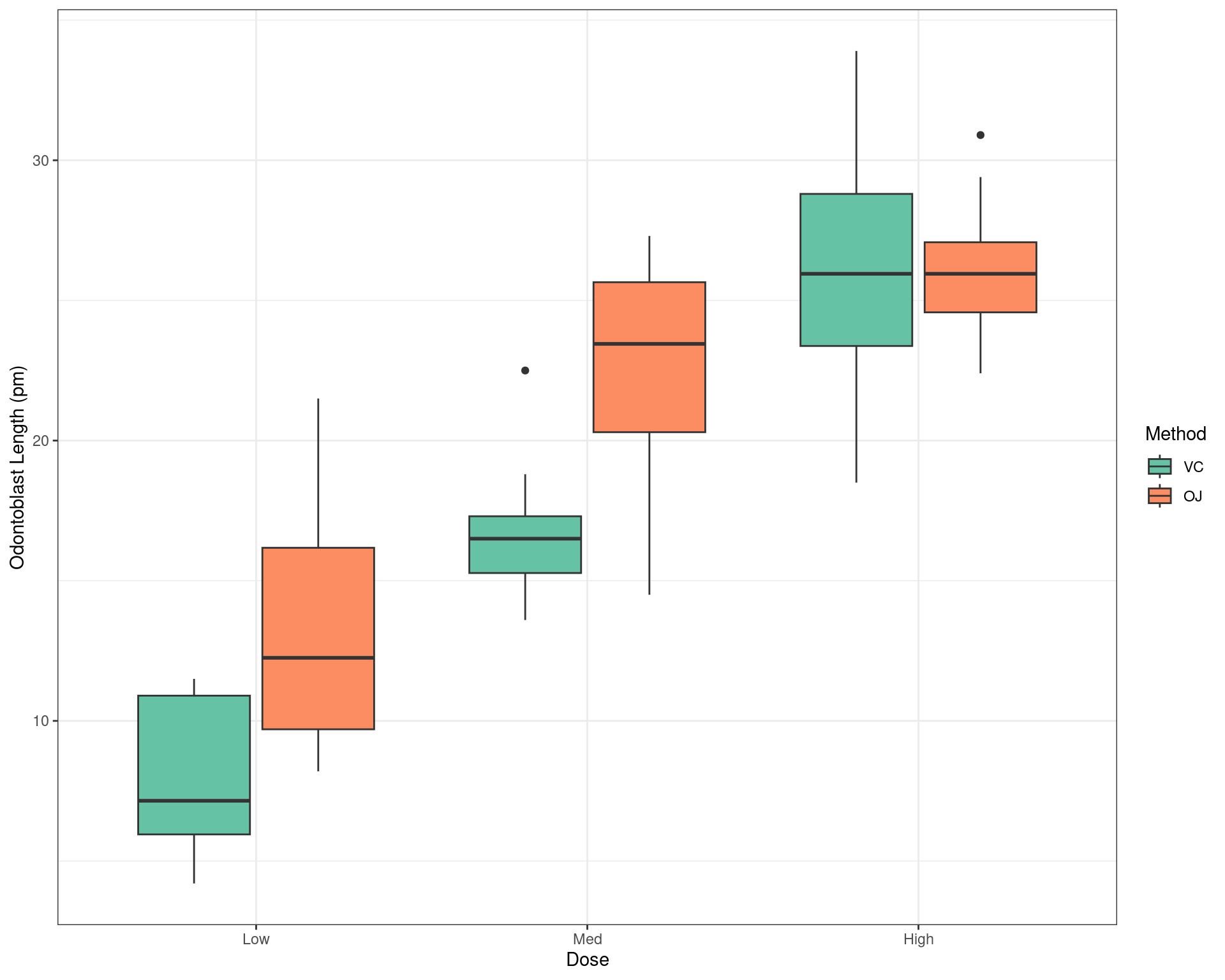
Visualising the Data

Type a description of the figure in the fig.cap section of the chunk header
- This will need to be placed inside quotation marks

My example text:

Odontoblast length shown by supplement method and dose level

Summarising Data

Next we might like to summarise the data as a table
- Show group means & standard deviations

Add the following to a new chunk called data-summary
- I’ve used the HTML code for $\pm$ (±)

pigs %>%
    summarise(
        n = n(),
        mn_len = mean(len), 
        sd_len = sd(len),
        .by = c(supp, dose)
    ) %>%
    mutate(
        mn_len = round(mn_len, 2),
        sd_len = round(sd_len, 2),
        len = paste0(mn_len, " &#177;", sd_len)
    ) %>%
    dplyr::select(supp, dose, n, len)

# A tibble: 6 × 4
  supp  dose      n len             
  <fct> <fct> <int> <chr>           
1 VC    Low      10 7.98 &#177;2.75 
2 VC    Med      10 16.77 &#177;2.52
3 VC    High     10 26.14 &#177;4.8 
4 OJ    Low      10 13.23 &#177;4.46
5 OJ    Med      10 22.7 &#177;3.91 
6 OJ    High     10 26.06 &#177;2.66

Knit…

Summarising Data

This has given a tibble output
We can produce an HTML table using pander

Add the following to your load-packages chunk

library(pander)

Producing Tables

pigs %>%
    summarise(
        n = n(), 
        mn_len = mean(len), 
        sd_len = sd(len),
        .by = c(supp, dose)
    ) %>%
    mutate(
        mn_len = round(mn_len, 2),
        sd_len = round(sd_len, 2),
        len = paste0(mn_len, " &#177;", sd_len)
    ) %>%
    dplyr::select(supp, dose, n, len) %>%
    rename_with(str_to_title) %>%
    pander(
        caption = "Odontoblast length for each group shown as mean&#177;SD"
    )

Producing Tables

Odontoblast length for each group shown as mean±SD
Supp	Dose	N	Len
VC	Low	10	7.98 ±2.75
VC	Med	10	16.77 ±2.52
VC	High	10	26.14 ±4.8
OJ	Low	10	13.23 ±4.46
OJ	Med	10	22.7 ±3.91
OJ	High	10	26.06 ±2.66

Analysing Data

Performing statistical analysis is beyond the scope of today BUT

The function lm() is used to perform linear regression

lm(len ~ supp + dose + supp:dose, data = pigs) %>%
    summary()


Call:
lm(formula = len ~ supp + dose + supp:dose, data = pigs)

Residuals:
   Min     1Q Median     3Q    Max 
 -8.20  -2.72  -0.27   2.65   8.27 

Coefficients:
                Estimate Std. Error t value Pr(>|t|)    
(Intercept)        7.980      1.148   6.949 4.98e-09 ***
suppOJ             5.250      1.624   3.233  0.00209 ** 
doseMed            8.790      1.624   5.413 1.46e-06 ***
doseHigh          18.160      1.624  11.182 1.13e-15 ***
suppOJ:doseMed     0.680      2.297   0.296  0.76831    
suppOJ:doseHigh   -5.330      2.297  -2.321  0.02411 *  
---
Signif. codes:  0 '***' 0.001 '**' 0.01 '*' 0.05 '.' 0.1 ' ' 1

Residual standard error: 3.631 on 54 degrees of freedom
Multiple R-squared:  0.7937,    Adjusted R-squared:  0.7746 
F-statistic: 41.56 on 5 and 54 DF,  p-value: < 2.2e-16

Analysing Data

pander can again be used to ‘tidy up’ the output from lm

lm(len ~ supp + dose + supp:dose, data = pigs) %>%
    summary() %>%
    pander(add.significance.stars = TRUE)

Analysing Data

	Estimate	Std. Error	t value	Pr(>\|t\|)
(Intercept)	7.98	1.148	6.949	4.984e-09	* * *
suppOJ	5.25	1.624	3.233	0.002092	* *
doseMed	8.79	1.624	5.413	1.463e-06	* * *
doseHigh	18.16	1.624	11.18	1.131e-15	* * *
suppOJ:doseMed	0.68	2.297	0.2961	0.7683
suppOJ:doseHigh	-5.33	2.297	-2.321	0.02411	*

Fitting linear model: len ~ supp + dose + supp:dose
Observations	Residual Std. Error	$R^2$	Adjusted $R^2$
60	3.631	0.7937	0.7746

Creating Summary Tables

Multiple other packages exist for table creation
- All do some things brilliantly, none does everything
pander is a good all-rounder
- Tables are very simplistic
- Also enables easy in-line results

Creating Summary Tables

To use other packages, $\implies$ broom::tidy()
- Will convert lm() output to a tibble
- This can be passed to other packages which make HTML / $\LaTeX$ tables

lm(len ~ supp + dose + supp:dose, data = pigs) %>%
    broom::tidy()

# A tibble: 6 × 5
  term            estimate std.error statistic  p.value
  <chr>              <dbl>     <dbl>     <dbl>    <dbl>
1 (Intercept)        7.98       1.15     6.95  4.98e- 9
2 suppOJ             5.25       1.62     3.23  2.09e- 3
3 doseMed            8.79       1.62     5.41  1.46e- 6
4 doseHigh          18.2        1.62    11.2   1.13e-15
5 suppOJ:doseMed     0.680      2.30     0.296 7.68e- 1
6 suppOJ:doseHigh   -5.33       2.30    -2.32  2.41e- 2

Creating Summary Tables

reactable creates amazing looking tables
DT also creates fantastic tables
- Less flexible with formatting
- Allows simple downloading to csv, xls etc.
gt is popular with some
xtable is excellent for $\LaTeX$ output

Complete the Analysis

After you’re happy with the way your analysis looks

A good habit is to finish with a section called Session Info
Add a code chunk which calls the R command sessionInfo()

So far we’ve been compiling everything as HTML, but let’s switch to an MS Word document. We could email this to our collaborators, or upload to Google docs

Summary

This basic process is incredibly useful

We never need to cut & paste anything between R and other documents
Every piece of information comes directly from our R analysis
We can very easily incorporate new data as it arrives
Source data is never modified
Creates reproducible research
Highly compatible with collaborative analysis & version control (Git)

R Markdown

R Markdown

Writing Reports Using rmarkdown

Writing Reports Using rmarkdown

Starting With Markdown

A Brief Primer on Markdown

Editing Markdown

Editing Markdown

Editing Markdown

Editing Markdown

R Markdown

Writing Reports Using rmarkdown

Writing Reports Using rmarkdown

Creating an R Markdown document

Creating an R Markdown document

Looking At The File

Looking At The File

Looking At The File

Getting Help

Compiling The Report

Compiling The Report

Compiling The Report

Making Our Own Report

Making Our Own Report

Making Our Own Reports

Making Our Own Reports

Creating a Code Chunk

Dealing With Messages

Dealing With Messages

Making Our Own Reports

Describing Data

Describing Data

Visualising The Data

Visualising the Data

Summarising Data

Summarising Data

Producing Tables

Producing Tables

Analysing Data

Analysing Data

Analysing Data

Creating Summary Tables

Creating Summary Tables

Creating Summary Tables

Complete the Analysis

Summary

Writing Reports Using `rmarkdown`

Writing Reports Using `rmarkdown`

Writing Reports Using `rmarkdown`

Writing Reports Using `rmarkdown`