A Brief Introduction to RNA-Seq

RAdelaide 2024

Dr Stevie Pederson

Black Ochre Data Labs
Telethon Kids Institute

July 11, 2024

Transcriptomic Analysis

Transcriptomic Analysis

• High-throughput transcriptomic analysis took off ~25 years ago
  • Followed the release of the the human genome very rapidly
• Microarrays enabled transcriptome-wide profiling of gene expression
  • Probes were designed for each targeted gene
• The Bioconductor package limma was first released in 2004 (Smyth 2004)
  • Still heavily used and maintained

• How does gene expression change across two or more groups
  • Control vs Treatment
• Represents an abundance analysis
• Relies on many, many cells pooled together

RNA-Seq

• The development of high-throughput sequencing \(\implies\) RNA-seq
• Rapidly replaced microarrays
• Needed fewer cells \(\implies\) could sample entire transcriptome

• Bulk RNA-Seq built on methods established for microarrays
  • New statistical models became quickly established
• Focussed on gene-level analysis
  • Now relatively mature

RNA-Seq

• Bulk RNA-Seq at the transcript level is still relatively immature
• Single-Cell RNA-Seq now has a degree of maturity
  • Cell trajectory analysis also moving rapidly
• Spatial Transcriptomics is an emerging and rapidly developing technology
  • Also includes imaging technologies

• Today we’ll focus on gene-level, bulk RNA-Seq analysis
  • Learning file types, packages, object classes, methods
  • Also visualisation strategies

Transcriptomes

• Genes are considered as genomic regions transcribed into RNA
• The complete region (i.e. locus) is transcribed
  • Introns are spliced out \(\implies\) mature transcripts

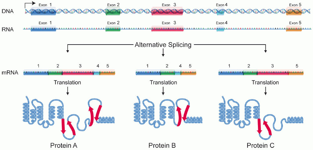
Image courtesy of National Human Genome Research Institute

Historically genes were considered to be units of heritability The idea of a transcribed locus is a modern concept

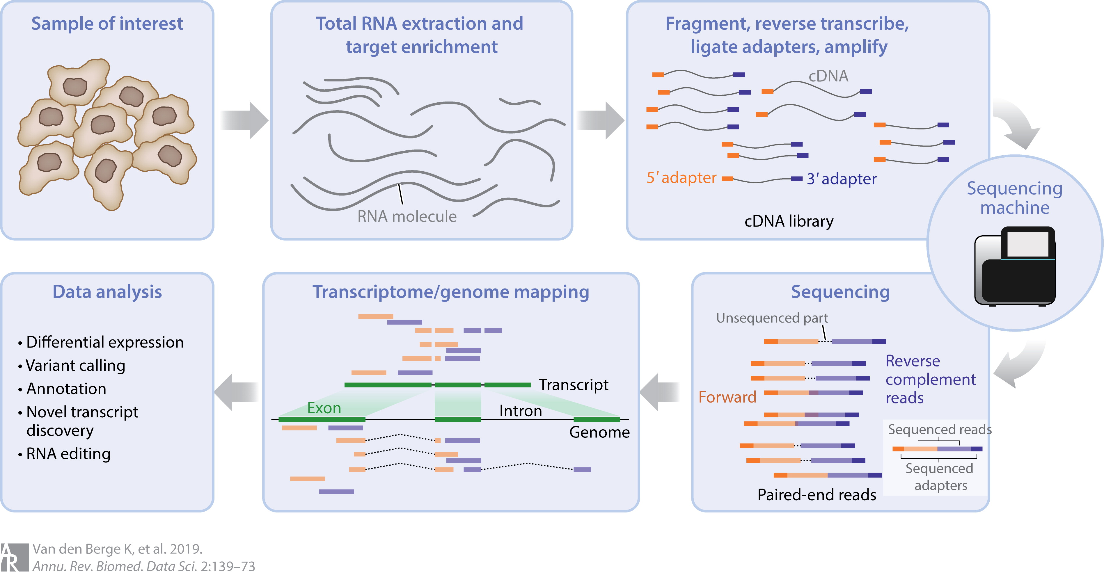
The Basics of Bulk RNA-Sequencing

1. Intact RNA is extracted from a sample
   • Tens of thousands of cells are lysed
   • May contain RNA from different cell types

2. RNA is fragmented into 250-500bp fragments
   • Lose short transcripts \(\implies\) long transcripts broken into pieces

The Basics of Bulk RNA-Sequencing

3. Prepared for sequencing
   • Converted to cDNA
   • Sequencing adapters added to all fragments
   • PCR amplification

4. Sequenced from both directions (paired end sequencing)
   • Commonly 50m reads/sample

The Basics of Bulk RNA-Sequencing

Sequencing Technology

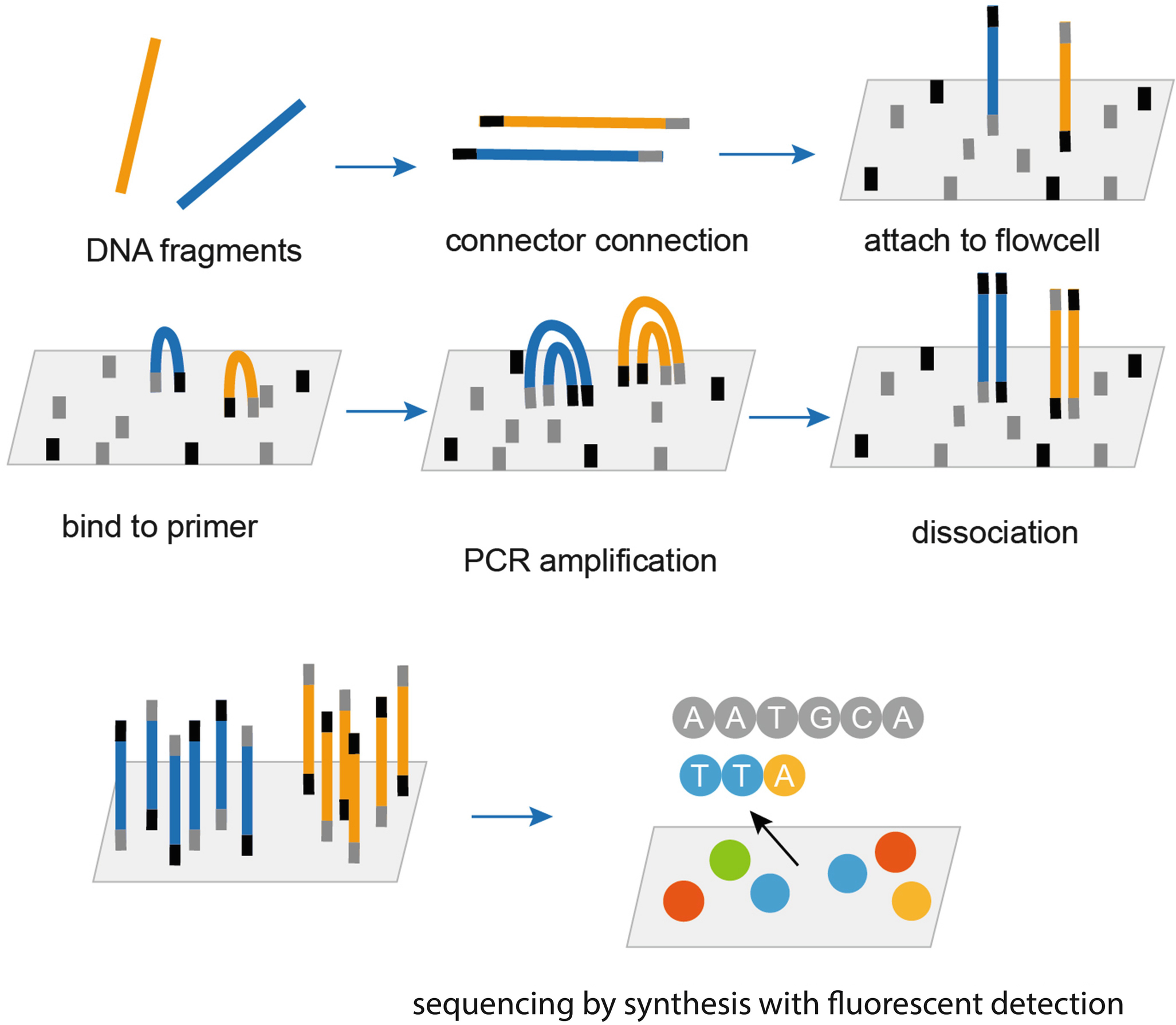
Wang, M. (2021). Next-Generation Sequencing (NGS). In: Pan, S., Tang, J. (eds) Clinical Molecular Diagnostics. Springer, Singapore. https://doi.org/10.1007/978-981-16-1037-0_23

• The prepared library is added to a flowcell
• Hopefully the dilution spreads molecules sparsely & evenly

Fastq Files

• The output from sequencing is a fastq file
  • Plain text file
• Commonly 30-50 million reads in each file
  • Each read takes 4 lines
  • 50m read x 4 lines = 200m lines
• Often compressed with fq.gz suffix
• Almost never parsed into R

Fastq Files

• If fragments are sequenced from one end only: single-end reads
• If sequenced from both ends: paired-end reads
• Both provided in separate files
  • {prefix}_R1.fq.gz + {prefix}_R2.fq.gz
  • Files match exactly
• Paired reads still represent a single fragment
  • More sequence information \(\implies\) more confident alignment

Fastq Files

1. Read header starts with @
2. Sequence
3. +
4. Quality scores

@SRR001666.1 071112_SLXA-EAS1_s_7:5:1:817:345 length=72
GGGTGATGGCCGCTGCCGATGGCGTCAAATCCCACCAAGTTACCCTTAACAACTTAAGGGTTTTCAAATAGA
+
IIIIIIIIIIIIIIIIIIIIIIIIIIIIII9IG9ICIIIIIIIIIIIIIIIIIIIIDIIIIIII>IIIIII/
@SRR001666.2 071112_SLXA-EAS1_s_7:5:1:801:338 length=72
GTTCAGGGATACGACGTTTGTATTTTAAGAATCTGAAGCAGAAGTCGATGATAATACGCGTCGTTTTATCAT
+
IIIIIIIIIIIIIIIIIIIIIIIIIIIIIIII6IBIIIIIIIIIIIIIIIIIIIIIIIGII>IIIII-I)8I

• We rarely parse these into R

Workflow Outline

1. QC and Read Trimming (optional) 😇

2. Align reads to the reference genome 😀
3. Count how many reads for each gene 😐
4. Statistical (DGE) analysis 😕
5. Enrichment analysis 😰
6. Biological Interpretation 😱

• Trimming, aligning and counting on an HPC
• QC analysis, Statistical and enrichment analysis in R
• Interpretation with domain experts

Counting is implemented in R but I generally don’t

Alternative Approaches

• Alternative methods align to transcript sequences NOT the genome
• These alignments are not spliced
• Most reads align to multiple transcripts
  • With genomic alignments usually a single alignment

• Transcript-level analysis is a newly solved problem (Baldoni et al. 2024)
• Downstream analysis using transcripts is challenging
  • Genes mapped to functions & pathways NOT transcripts

Data Pre-Processing

• A ‘read’ is the total signal from an entire cluster of molecules
• If errors occur during cluster formation:
  • Molecules get ‘out-of-sync’
  • Actual sequence becomes uncertain
  • Low quality scores assigned
• Most people discard low quality reads
• Adapter sequences at either end can also be removed
  • Derive from short RNA fragments

Data Pre-Processing

• Overall summaries of library quality can be obtained \(\implies\) FastQC
• Multiple tools to perform Pre-processing
  • cutadapt, AdapterRemoval, trimmomatic, TrimGalore etc
  • Potentially problematic reads or sequences removed
• fastp combines QC reports with read trimming

Data Pre-Processing

• FastQC, fastp, cutadapt all return reports after running
  • Are run on a single library (i.e. sample) at a time
• MultiQC is an excellent standalone tool for combining all reports
• ngsReports is the “go-to” Bioconductor package for this
  • Can also import alignment summaries + many others

Not going to go into ngsReports today but I use regularly in my QC workflows

Alignment

• Pre-processed reads are aligned to a genome
• All aligners based on Burrows-Wheeler Transform
  • Comp. Sci algorithm for fast searching
  • Requires the creation of an index which is searched
• Most common aligners are STAR, hisat2 or bowtie2
  • All splice-aware
  • GTF used during building of the index
• Requires an HPC & scripting skills

Bam Files

• After alignment to the reference \(\implies\) bam files produced
• Usually contain millions of alignments
• Each read now occupies a single line with 11 tab-separated fields

Column	Field	Description
1	QNAME	The original FastQ header line
2	FLAG	Information regarding pairing, primary alignment, duplicate status, unmapped etc
3	RNAME	Reference sequence name (e.g. chr1)
4	POS	Left-most co-ordinate in the alignment
5	MAPQ	Mapping quality score
6	CIGAR	Code summarising exact matches, insertions, deletions etc.
7	RNEXT	Reference sequence the mate aligned to
8	PNEXT	Left-most co-ordinate the mate aligned to
9	TLEN	Read length
10	SEQ	The original read sequence
11	QUAL	The read quality scores

SAM files are plain text whilst BAM are compressed to save storage

Bam Files

• 12th (optional) column often contains tags
  • NH:i:1 indicates this read aligned only once
  • AS:i:290 the actual alignment score produced by the aligner
  • NM:i:2 two edits are required to perfectly match the reference

• Reads can align to multiple locations
  • Sometimes more alignments than reads
• Rarely, only one read in a pair may align
• Generally view small subsets of data using samtools in bash

Bam Files

• The Bioconductor interface to bam files is Rsamtools
• We define BamFile or BamFileList objects
• Are a simple connection to the file (including checks)
• We don’t load anything when created
  • Instead define specific subsets to load for a specific task

Bam Files

• When loading a subset of reads set ScanBamParam()
• Enables loading alignments:
  • from specific ranges (using GRanges)
  • with specific tags or flags
• Controls which columns are returned

• Sequences loaded as DNAStringSets
• Alignment co-ordinates as GRanges objects

Read Counting

• Most assigning of reads to genes is performed by external tools
• Gene, Transcript & Exon co-ordinates passed in a GTF
  • Aligned Reads overlapping an exon/transcript/gene are counted

• Produces flat (i.e. tsv) files \(\implies\) count once & load each time you start
• Today’s count data produced using featureCounts from the Subread tool
  • Other tools are RSEM, htseq

Read Counting

• Counting can be performed in R:
  • Rsubread or GenomicAlignments
• Should still only be performed once and saved as a standalone file
  • Would avoid doing at the start of every R script

Reference Annotations

• Reference genomes are relatively stable over many years
• Available from multiple sources
  • Inconsistent use of the “chr” prefix
  • Inconsistency in “chrM” or “chrMT”
  • Some variability in scaffolds

Reference Annotations

• Annotation sets are updated multiple times every year
  • Gencode, Ensembl, UCSC
  • Usually minor changes
• Not important for genomic alignment
• Very important for read counting & transcriptomic alignment

• Changes appear as genes move from predicted to verified
• Prediction algorithms also change

Reference Annotations

• The latest Gencode set of annotations (Release 46, May 2024)
• 63,086 Genes
  • 19,411 protein coding
  • Remainder are lncRNA, pseudogenes etc
• 254,070 Transcripts
  • 89,581 protein coding
  • Remainder are NMD, lncRNA etc
• Shortest annotated (spliced) transcript is 8nt \(\implies\) longest is 350,375nt

Checking Gencode v41 there were 251,295 transcripts and 61,906 genes

References

Baldoni, Pedro L, Yunshun Chen, Soroor Hediyeh-Zadeh, Yang Liao, Xueyi Dong, Matthew E Ritchie, Wei Shi, and Gordon K Smyth. 2024. “Dividing Out Quantification Uncertainty Allows Efficient Assessment of Differential Transcript Expression with edgeR.” Nucleic Acids Res. 52 (3): e13.

Smyth, Gordon K. 2004. “Linear Models and Empirical Bayes Methods for Assessing Differential Expression in Microarray Experiments.” Stat. Appl. Genet. Mol. Biol. 3 (February): Article3.